Summary
In this post, I do climate year classifications on BEC variants at the provincial scale. I test the performance of variations on four distinct classification methods: nearest-neighbour classification, linear discriminant analysis, quadratic discriminant analysis, and Random Forests. Quadratic discriminant analysis is the clear winner, though the poor performance of Random Forests deserves a closer look. I do some simulations to illustrate the behaviour of these different methods. I establish that the “curse of dimensionality” is not apparent in this analysis, except for Random Forests. Finally, I provide a summary of QDA classification by BEC zone, indicating that BEC zones of the southern and central interior have significantly lower differentiation than those of the coast and northern interior.
Take-home message: QDA is much more powerful than PCA nearest neighbour classification at defining climatic domains of BEC variants (79% vs. 36% correct classification rate, respectively). This indicates that mahalanobis distance metrics (e.g. nearest neighbour on standardized variables, standard deviation of z-scores) are not sufficient to quantify climatic differentiation in a temporal climate envelope analysis. A more sophisticated distance metric is likely required for temporal climate envelope analysis.
Introduction to Climate Year Classification
A climate year classification applies a climate classification scheme to the variable climatic conditions of individual years at a single location, rather than to spatial variability of climate normals. This approach can be applied to BEC variants. The characteristic conditions of BEC variants can be identified as the centroid of their spatial variation in a set of climate normals. The individual years of the normal period at a location representing that centroid (the “centroid surrogate”) can then be classified based on their relative similarity to the conditions of the centroids.
Unsupervised classification using supervised classification procedures
Typical supervised classification procedures split data with known classes into training data and test data. The training data are used to parameterize the classification model, and the test data are used to evaluate the effectiveness the model. In supervised classification, the proportion of test observations that are correctly classified is a definitive criterion for model effectiveness. The correct classification rate indicates the degree of confidence with which the model can be used for “predictive” classification of new data with unknown classes.
In contrast to this conventional supervised classification approach, the objective of climate year classification is description, rather than prediction. Climate years have an a priori identity: the BEC variant of the centroid surrogate that they belong to. However, the actual class of the climate year is not known a priori. A confusion matrix in this context is a description of the characteristic conditions (in terms of BEC variants) of the climate years for each BEC variant centroid surrogate. In this context, classification “error” is a misnomer since the class of the climate year is not known a priori. Nevertheless, correct classification rate—the proportion of the climate years of a BEC variant that are classified as that BEC variant—is an ecologically meaningful measure of the climatic differentiation between BEC variants. In this way, climate year classification uses the validation tools of supervised classification—confusion matrices and correct classification rates—as the descriptive outputs of an unsupervised classification of climate years.
Climatic domains of BEC variants
Most classification algorithms assign classes to observations based on decision boundaries in the data space. Each class therefore is associated with a hypervolume (contiguous region of the data space), and all observations that fall into that region will be assigned to that class. In climate year classification, this hypervolume can be thought of as the “domain” of the BEC variant. BEC variants are map units of ecologically significant differences in climate, so the shape of this domain reflects to some extent the thresholds of ecological response to climate variation. However, the shapes of the domains also reflect to some extent the quality of the BEC mapping.
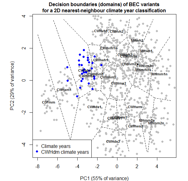
Figure 1: illustration of the BEC variant “domain” concept in climate year classification. In this simplified example of a nearest-neighbour classification in two dimensions, domain boundaries are lines of equal distance between BEC variant climatic centroids.
The climatic domain concept in is illustrated in Figure 1. For simplicity, this illustration shows a nearest-neighbour climate year classification in a two-dimensional climate space. There are several attributes of this illustration that apply to climate year classification in general:
- The BEC variant’s climatic centroid is rarely at the centroid of the BEC variant’s domain. in this illustration, the centroid of the CWHdm is very close to the domain boundary, due to the proximity of the CWHxm2 centroid. This proximity may reflect true ecological thresholds, errors in the BEC itself, or insufficient dimensionality of the climate space.
- Domains are unbounded for BEC variants on coastal (e.g. CWHvh1), elevational (e.g. MHwh1), or political (e.g. CDFmm) boundaries. This creates the potential for misclassification of novel climatic conditions and highlights the need for additional decision boundaries to bound the domains of BEC variants on all sides.
- The climate space is not fully occupied. For example, there is a gap between the CWHwm and the MHmm1s. this gap may indicate climatic conditions that are truly absent from the landscape, or BEC units that are defined too broadly.
Candidate methods for climate year classification
Correct classification rate depends on many factors: (1) climate year variability relative to the distance to adjacent centroids, (2) whether the domain is bounded on all sides, and (3) whether the climate space includes the necessary dimensions of differentiation. In addition, classification method is an important consideration in ensuring that BEC variant domains are appropriately defined. The following classification methods are evaluated in this analysis:
- nearest-neighbour classification on standardized raw variables (“raw”)
- nearest-neighbour classification on principal components (“pca”)
- linear discriminant analysis (“lda”)
- nearest-neighbour classification on linear discriminants (“nnlda”)
- linear discriminant analysis on principal components (“ldapc”)
- linear discriminant analysis without normalization of within-groups covariance (“diylda”)
- quadratic discriminant analysis (“qda”)
- Random Forests (“rf”)
Some of these methods are theoretically equivalent, but nevertheless were included in the analysis to verify this equivalency in practice.
The data for this analysis are the 1961-1990 climate years at the 168 centroid surrogates representing forested BEC variants in British Columbia. I used 14 annual climate elements as the raw variables: MAT, MWMT, MCMT, TD, MAP, MSP, AHM, SHM, DD_0, DD5, FFP, PAS, Eref, and CMD. I log-transformed precipitation and heat-moisture variables (MAP, MSP, AHM, SHM, PAS) to normalize their distributions. All variables were standardized to a mean of zero and variance of 1.
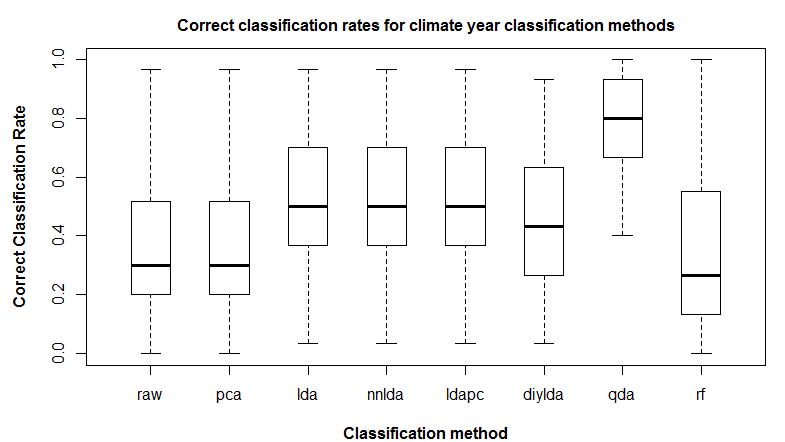
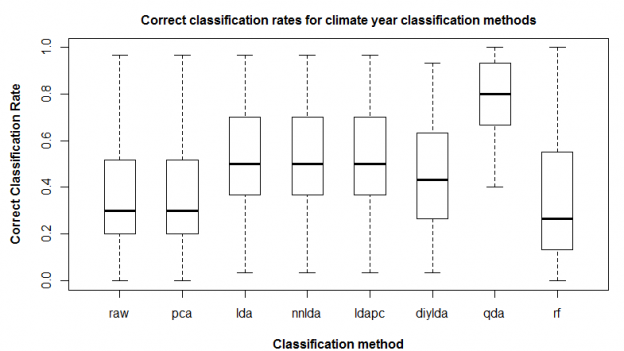
Figure 2: comparison of correct classification rate (proportion of climate years in home domain) for eight classification methods: nearest-neighbour on standardized raw variables (“raw”); nearest-neighbour on principal components (“pca”); linear discriminant analysis (“lda”); nearest-neighbour on linear discriminants (“nnlda”); linear discriminant analysis on principal components (“ldapc”); linear discriminant analysis without normalization of within-groups covariance (“diylda”); quadratic discriminant analysis (“qda”); and random forests (“rf”).
Figure 2 shows correct classification rate for each of the classification methods. The following observations are notable:
- Nearest neighbour classification returned identical results on the raw standardized variables and the principal components. This is logical since PCA does not perform a transformation of the data, only a rotation of the axes.
- LDA outperforms PCA substantially. Since all features were retained for both classifications, the superiority of LDA is not due to better feature extraction. Instead, it is because the coefficients of the linear discriminants incorporate a transformation of the data based on the ratio of between-groups to within-groups variance.
- The results of lda, nnlda, and ldapc classification are the same. This indicates that the predict(lda()) function in R is simply performing a nearest-neighbour classification on the linear discriminants. It also indicates that LDA on the PCs is functionally equivalent to LDA on the raw data.
- LDA without spherical normalization of the within-groups covariance matrix (“diylda”) has intermediate performance between LDA and PCA, indicating that SW normalization is an important component of LDA classification.
- QDA vastly outperforms all of the other methods. This indicates that the within-groups covariance matrices are unequal, and also suggests that non-linear decision boundaries are more appropriate for these data.
- Random Forests had the poorest median performance of all the methods. This is surprising, given that Wang et al. (2012) found that Random Forests outperformed LDA on a classification of spatial variation of climate normals. This poor result may be due to the use of default parameters in R, and should be investigated further.
Simulations of PCA, LDA, QDA, and Random Forests
To illustrate the behaviour of the four distinct classification methods, they were applied to simulated two-dimensional data of three groups with unequal within-groups covariance matrices (Figure 3). In this case, LDA provided a marginal improvement over nearest-neighbour classification. QDA provided a substantial improvement, due in part to the ability of the method to discern groups with different variance but also due to the use of a parabolic decision boundary between groups 1 and 2. Random Forests doesn’t use a decision boundary, which is evident in two bizarre misclassifications in the core domains of groups 1 and 2.
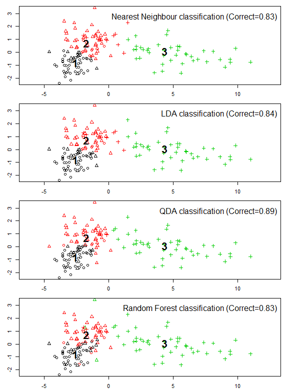
Figure 3: classifications of simulated two-dimensional data, illustrating the behaviour of nearest-neighbour classification, linear discriminant analysis, quadratic discriminant analysis, and Random Forests. Point symbols are the a priori identity of the data, and colours are the classes assigned by the classification methods.
Is the curse of dimensionality at play?
To avoid artefacts of dimension-reduction, all classifications in this trial were performed on full-dimensional data, i.e. where feature extraction is performed, all features are retained. There are 14 raw variables, and 14 extracted features. This approach raises the spectre of the “curse of dimensionality”. This term generally refers to the prohibitive sample sizes required to infer statistical significance in high-dimensional data. However, effective data sparsity may also affect inferences of similarity. To test the effect of dimensionality on climate year classification, I performed climate year classifications on reduced climate spaces composed of 2 to 14 extracted features (Figure 4). QDA and Random Forests were performed on linear discriminants, for simplicity in the case of the former and by necessity in the case of the latter.
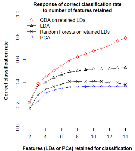
Figure 4: Response of correct classification rate to number of features retained. This result indicates the “curse of dimensionality” is not evident in the classifications, except for a subtle effect in Random Forests.
All classification methods except for Random Forests respond positively to increasing number of features, indicating that the curse of dimensionality is not at play in these methods at this scale of dimensionality. Random forests exhibits a decline in correct classification rate after 9 dimensions, suggesting that it is more sensitive to dimensionality than the other methods. The consistent incremental response of QDA to increasing dimensions is striking, and suggests that addition of more raw variables could improve classification further. However, this result is likely due to the use of linear discriminants as the input data to QDA. This test could be refined by projecting the data onto quadratic discriminants.
QDA classification summaries for BEC zones
One of the purposes of climate year classification is to understand the relative climatic differentiation in different regions of the province. Low differentiation in a BEC zone suggests that BEC mapping is at a finer climatic scale, either because plant communities are more sensitive to subtle climatic differences, or because mapping approaches differed amongst regional ecologists responsible for the BEC mapping.
Figure 5 indicates that the southern and central interior BEC zones have lower differentiation than the coastal and northern interior zones. It is likely that this effect would be even more pronounced if the classification was controlled for unbounded domains.
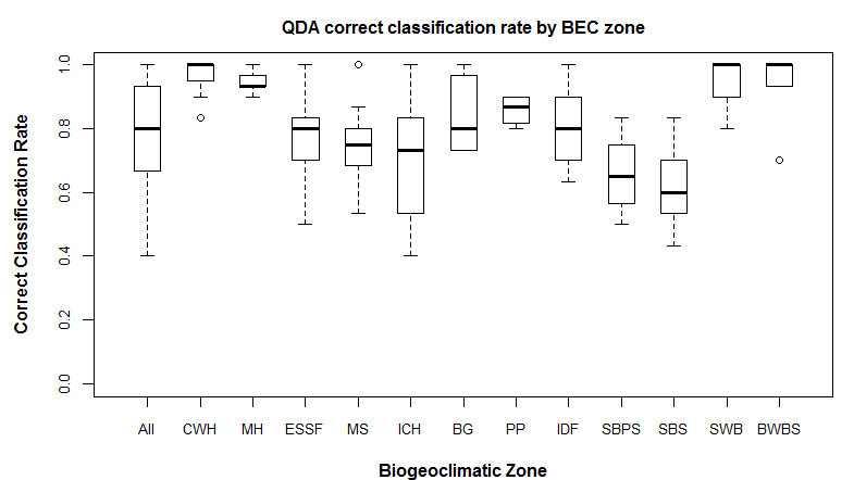
Figure 5: QDA correct classification rate, summarized by BEC zone. The coastal (CWH/MH) and northern interior (SWB and BWBS) regions have higher correct classification rates than the southern and central interior regions.
Possible Next Steps
- Develop a method for controlling for unbounded domains. This will likely involve applying a boundary to a certain distance (e.g. group-specific standard deviation) from each group centroid. This approach will allow identification of novel conditions.
- Investigate any limitations of QDA for climate year classification.
- Verify the poor performance of Random Forests.
- Test the methods on a high-dimensional data set (e.g. all monthly variables).
References
Wang, T., E. M. Campbell, G. A. O’Neill, and S. N. Aitken. 2012. Projecting future distributions of ecosystem climate niches: Uncertainties and management applications. Forest Ecology and Management 279:128–140.