Summary
Climate change trends must be removed from the interannual variability used to determine temporal climate envelopes, otherwise locations with rapid historical climate change would be interpreted as having greater background variability. However, the climate system is too complex to expect that there will be an objective division between trend and variability; an arbitrary distinction must be made. Empirical mode decomposition (EMD) (Huang et al. 1998) extracts intrinsic and adaptive trends from non-linear and non-stationary time series. In contrast to other intrinsic/adaptive methods such as locally weighted regression, EMD is appealing because it is the implementation of an explicit definition of trend. The results from this evaluation suggest that EMD is a viable method for removing the trend from historical climatic variability, though further refinement and testing are required to ensure that it is implemented appropriately. Detrending is shown to have a dramatic effect on climate year classification: there appears to be almost no overlaps in detrended climate envelopes of BEC variants.
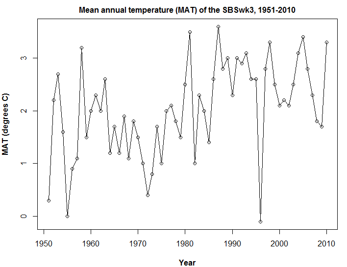
Figure 1: A time series of mean annual temperature in British Columbia’s central interior plateau. The differentiation of interannual variability from the long term climate change trend is not straightforward.
Distinguishing trend from variability
The premise of the temporal climate envelope approach is that interannual climatic variability at any given location provides a scale for assessing the ecological significance of climate change in both space and time. However, this approach requires that a distinction must be made between interannual variability and climate change. In order for the interannual variability to be quantified, the climate change trend must be removed. The methodology for removal of the trend can be a critical consideration for climate change analysis, because it implicitly defines what will be considered climate change as opposed to background variability.
The time series of mean annual temperature in British Columbia’s central interior plateau (Figure 1) demonstrates that detrending is essential to analysis of interannual variability. Without detrending, regions with more rapid historical climate change will be spuriously assigned a higher range of interannual climatic variability than regions with less historical climate change. This would confound an assessment of the ecological significance of climate change based on historical variability. However, the MAT time series suggests that there is no clear distinction between interannual variability and long term climate change. Oscillations are apparent, but they occur on a continuum of magnitudes and frequencies.
Wu et al. (2007) provide an excellent characterization of the problem of trend identification in climate data. They first explicitly define the term trend as an attribute specific to an arbitrary time scale: “The trend is an intrinsically fitted monotonic function or a function in which there can be at most one extremum within a given data span.” Their definition of variability follows: “the variability is the residue of the data after the removal of the trend within a given data span.”
They note that due to the complexity of the global climate system, climate time series must be expected to be non-linear and non-stationary. in light of this expectation, Wu et al. (2007) make a distinction between extrinsic/predetermined methods for trend identification and intrinsic/adaptive methods. Extrinsic methods—including linear and non-linear regression, classical decomposition, and moving averages—impose a predetermined functional form onto the data and therefore are inappropriate for nonlinear non-stationary time series. Wu et al. (2007) advocate for intrinsic methods that are adaptive to the changing attributes of the signal throughout the time series. Specifically, they suggest empirical mode decomposition (EMD) (Huang et al. 1998) as the only method able to adequately determine the trend in nonlinear non-stationary time series.
Empirical mode decomposition (EMD)
EMD decomposes time series into intrinsic mode functions (IMFs), which are oscillations of various time scales that (1) have extrema and zero-crossings that differ in number only by one, and (2) have equal absolute mean values of minima and maxima. The residual of this process is a monotonic function with only one set of extremes, which is the trend as they previously defined it. EMD is an appealing approach for detrending variability. It is very widely cited (3320 citations in web of science), and deserves evaluation.
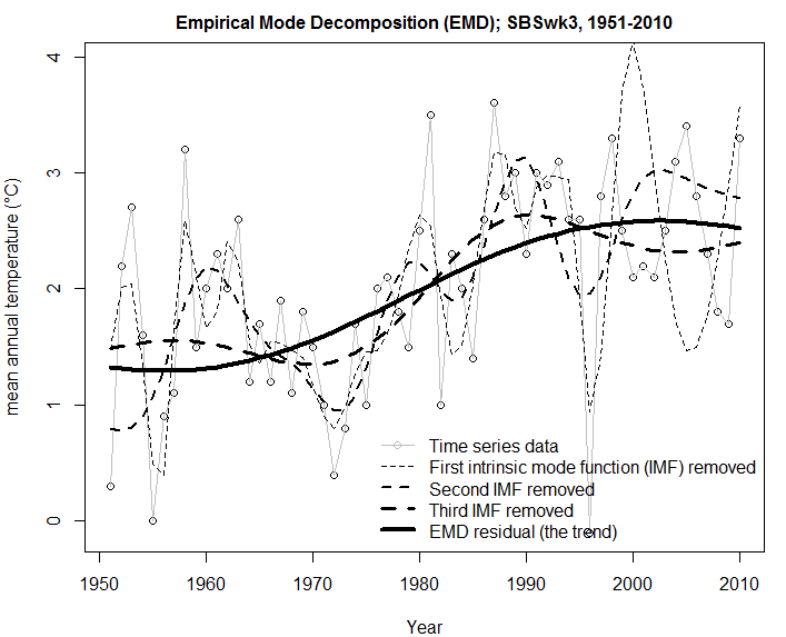
Figure 2:A demonstration of empirical mode decomposition (EMD) on the SBSwk3 MAT time series. This process was performed using the emd(y,x) command in R, with default parameters.
Figure 2 is a demonstration of EMD on the SBSwk3 MAT time series, using the emd(y,x) call in R with default parameters. There are some problematic features of the decomposition. For example, the prominent oscillation in the raw data from 1998 onwards seems to be very poorly decomposed: the removal of the first IMF puts subsequent IMFs out of phase and out of scale with this oscillation. This is likely an example of “mode-mixing”, which is cited as a common problem with EMD. However, the residual trend does not appear to be affected. Another potential critique of the residual trend is that it is out of phase with the dominant oscillation between 1950 and 1970. However, this is consistent with the explicit definition of trend in Wu et al. (2007); i.e. that a trend is a monotonic attribute of a given time span. Any oscillations over shorter time periods are explicitly considered be variability. This highlights the importance of choosing a time span that is meaningful to the interpretation of the variability and the trend.
EMD provides reasonable trend extraction over the 14 annual climate variables that I am currently using for my research (Figure 3). The EMD trends are similar to locally weighted linear regression (LOWESS), which is also an intrinsic/adaptive means of trend extraction. The main advantage of EMD over LOWESS is that EMD implements an explicit definition of trend that is free of local influences. However, EMD exhibits undesirable behaviour in the time series of mean summer precipitation (MSP), where it appears to exaggerate a very subtle trend. This undesirable behaviour appears to be primarily limited to the beginning and end of the time series. For this reason, it is likely necessary to exclude some outer portion of the time span from the temporal climate envelope. Further exploratory work is required to ensure that I am implementing the method to its full potential.
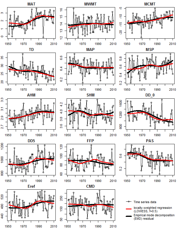
Figure 3: Trends extracted by EMD from the time series of 14 annual climate variables at the SBSwk3 centroid surrogate. Another intrinsic/adaptive trend extraction, LOWESS, is shown for comparison.
Effect of detrending on climate-year classification
Detrending reduces the interannual variability at any given location, and therefore will reduce overlaps of temporal climate envelopes. As a result, it is logical that detrending will improve differentiation of BEC variants in a climate year classification. This effect is demonstrated in Figure 4. Notably, quadratic discriminant analysis achieves almost perfect differentiation on the detrended data (97% correct classification rate on average). This is a remarkable result, given that preliminary results using linear discriminant analysis on raw data suggested that there was approximately 50% overlap in BEC variant temporal climate envelopes. Since quadratic discriminant analysis classifies based on decision boundaries, the classification of detrended data indicates that there is almost no overlap in BEC variant temporal climate envelopes.
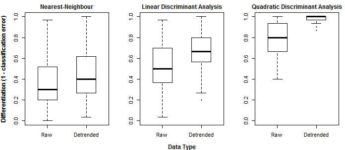
Figure 4: Effect of detrending on climate year classification results for the 1961-1990 normal period.
Effect of detrending on feature extraction (PCA)
Detrending applies a different scalar to each year of each location (i.e. BEC variant centroid surrogates) in the spatiotemporal data. As a result, detrending is an alteration of the structure of the data. However, this distortion appears to be subtle (Figure 5). Detrending increases the eigenvalues of the last 4 PCs This likely is due to decorrelation of derived climate variables: the trends extracted add some noise to the relationship between the independent variables (e.g. MAT, MAP) and derived variables (e.g. DD5, Eref).
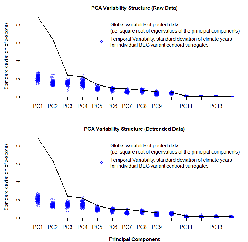
Figure 5: Effect of detrending on the variability structure of the multivariate climate space (1961-1990 data).
Appropriate time span for trend extraction
Consistent with their definition of trend, Wu et al. (2007) note that trends extracted by EMD are dependent on the time span of the data. This raises the issue of the appropriate time span to use for detrending of temporal climate envelope data. So far, I have used a time span of 1951-2010 (60 years) because this is the period of most reliable weather station data. However, temporal climate envelopes will very likely be developed for normal periods (30-year time span), so it is reasonable to consider using 30 years as the time span for trend extraction.
EMD trends for 30- vs. 60-year periods are compared in Figure 6. EMD exhibits some erratic behaviour at the beginning and ending of the 30-year time spans, i.e. unsupported upswings or downswings. However, even in cases where it behaves appropriately on 30-year time spans (e.g. MCMT), it extracts oscillations could reasonably be considered to be part of background (non-trend) climatic variability. This demonstration indicates that, using EMD or any other method, normal periods are likely too short for trend identification. 60 years appears to be a necessary time span for trend extraction, even though detrended temporal climate envelopes are calculated from 30-yr normal periods.
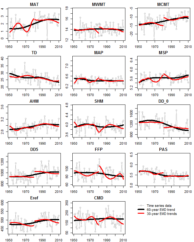
Figure 6: Comparison of EMD trend extraction over 30- vs. 60-year time spans of the time series of 14 annual climate variables at the SBSwk3 centroid surrogate.
References
Huang, N. E., Z. Shen, S. R. Long, M. C. Wu, H. H. Shih, Q. Zheng, N.-C. Yen, and C. Chao. 1998. The Empirical Mode Decomposition and the Hilbert Spectrum for Nonlinear and Non-Stationary Time Series Analysis. Proceedings of the Royal Society London 454:903–995.
Wu, Z., N. E. Huang, S. R. Long, and C.-K. Peng. 2007. On the trend, detrending, and variability of nonlinear and nonstationary time series. Proceedings of the National Academy of Sciences of the United States of America 104:14889–94.