Brower, A., & Carrol, L. (2007). Spatial and Temporal Aspects of Alcohol-Related Crime in a College Town. Journal of American College Health, 55(5), 267-276.

This paper looked at alcohol-related crime (vandalism, assault and battery, liquor law violations, and noise complaints) in Madison, Wisconsin. Madison has a large university student population known for their high alcohol consumption – rate of binge-drinking of 63% (2007), vs. US national average of 44%. The researchers wanted to look at the spatial and temporal distribution of these crimes to link them to student binge-drinking.

The researchers’ hypothesis was that:

• Alcohol-related crimes will display certain temporal and spatial patterns that prove their connection to student binge-drinking, such as noise complaint calls to the police made from households neighboring high-density student areas at around midnight

Methods

Two Data Sets gathered:

• Student Addresses from students registered in 2003 (from University of Wisconsin)

• Alcohol-related crime calls to the police(from Madison PD and UW PD) in 2003

The results were mapped in ArcGIS, with a focus on downtown Madison, producing several maps: areas with high student populations; spatial distribution of crimes; crime locationsat the time when different type of crime peaked (e.g. noise complaints from 11 PM to midnight), as well as a graph showing the temporal (hourly) fluctuation in each crime type.

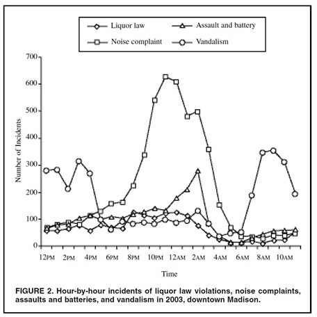
Temporal crime fluctuations

Results

Several spatial and temporal patterns identified:

noise-complaints calls peaked around 11pm to midnight in areas bordering high student population areas

Assault and Battery reports peaked at 2-3 AM when bars closed down

Vandalism peaked in morning (time when the crime was discovered and reported), and was concentrated around areas with high student populations

Researchers thus found support for their hypothesis.

Limitations

• Incomplete analysis – e.g. did not talk about spatial distribution of assault and battery crimes
• Crimes may have been called in multiple times; others may have not been represented at all because the police responded first
• Poorly-produced maps – poor use of colors and symbols, unclear what exactly some maps showed
• Did not map bar locations
• Made several assumptions, such as that students are the main demographic at bars
• Could have mentioned whether drinking-related crime rates are high or not

Rating: 5/10 – weak paper, but it did lead to policy changes by city and university officials in regards to binge-drinking

GIS and Crime

There is some controversy in the crime field in regards to how important/useful environmental considerations are. Some crime specialists believe geography/the environment don’t play a big role.

Example of GIS/Crime:

Greed/Envy/Wrath maps of the US:

Greed shows average income compared with number of people below poverty line

Envy – total thefts per capita

Wrath – number of violent crimes per capita

Routine activities theory (RAT):

Theory that crime is based on routines – both of the criminals and the targets. This theory highlights temporal and socioeconomic aspects of crime, but does not consider the spatial, and thus geographical aspect.

Crime Pattern Theory:

Crimes tend to happen in certain neighborhoods because that’s where the criminals live.

Environmental criminology

Environmental criminology is a related sub-discipline that considers the spatial distribution of offenses and offenders.

Marauders vs. Commuters

Example of geography use in crime:

Picton murders – Kim Rossmo figured out that the Picton murders were commuted by a serial killer, but it took 5 years to actually figure out it was Picton, because nobody would listen to him. Kim is a pioneer of geographic profiling.

This was our second week of presentations, this time looking at Health Geography rather than landscape ecology. My paper looked at the relationship between residential slopes and likelihood of diabetes in Perth, Australia.

Paper reviewed: People living in hilly residential areas in metropolitan Perth have less diabetes: spurious association or important environmental determinant?

Focus of study: Built Environment Factors that affect Diabetes prevalence

Research question: Is there a link between neighborhood slope and likelihood of having diabetes?

Researchers’ Hypotheses:

• People that live in higher-slope areas will have a smaller chance of contracting diabetes, due to higher exertion during any physical activity, such as walking

Methods:

• West Australia 2003-2009 Health Survey data – 11,406 individuals / 964 with Diabetes
• Physical location of every individual -> created 1600m long neighborhood around every home
• 90m DEM map of Perth showing slope placed on top
• 5 groups of confounding variables also collected: socio-economic, distance to important destinations, walkability, diet, amount of time walking

Analysis:

• SPSS software program used to look association between slope and diabetes, and also between diabetes and confounding factors
• 5 models produced, each accounting for more of the confounding factors

Results:

• Strong association found between slope and diabetes, even after accounting for confounding variables – 13% lower odds of having diabetes for every 1% increase in mean slope

Conclusion:

• Paper had many limitations
• The researchers don’t explain how adjusting for confounding factors was done
• association could be false, caused by confounding factors
• slope for each neighborhood was averaged out, may not represent actual walking route slope
• could’ve employed GWR
• 7/10

Other presentations:

The one thing that really struck me with this round of paper reviews is how similar they were in format. For example, a lot, if not most of the papers had Odds Ratios within a Confidence Interval to show relationships, rather than correlation coefficients. Another trend I noticed is that the researchers focused a lot on their own limitations.

It seems like research in Health Geography is focused on trying to be as careful as possible when making conclusions from their research, and looking at association rather than causation, because of how complex health-related issues are.

GIS in health geography

This lecture follows up from the health geography lecture from last week. The goal of this lecture is to consider all of the nuances related to using GIS and health geography, and to provide examples of GIS and health geography.

Spatial epidemiology is arguably the biggest application/subfield of health geography. It seeks to understand and describe the spatial variation of diseases. It draws largely upon ego-referenced health and population data kept by governments – e.g. recorded information about an individual’s visit to the doctor. Spatial epidemiology is largely focused on the individual level and small areas; otherwise it is impossible to see how diseases originate, spread, and so on.

Some Issues

Aligning different spatial units is difficult for GIS and health geography -e.g. different sizes/boundaries for various types of administrative districts. Data on population movement is also difficult to find – e.g. people migrating over long time periods, as well as daily movements.

Environmental hazards are a big component of GIS in health geography, because they can be mapped well.

Health Geography

The topic for today’s lecture is Geography and Health. Because spatial location is a very big factor for health-related concerns, such as children living near a highway having higher chance of developing asthma, geography (and more specifically, GIS) is a very useful discipline for examining and treating health issues. John Snow’s 1854 map of a cholera outbreak in London is a classic example of the intersection of spatial geography and health – the map showed that cholera was caused by contaminated water ended up changing public policy. Another way geography is useful to health is figure out the ideal way to provide medical services – e.g. figuring  out the ideal hospital to accept people from a far away town.

Another classic example is a map showing changes in rates of obesity, usually between different states in different time periods in the United States.

Another related concept is Medical Geography – the application of geographical perspectives to investigate health-related topics. Medical geography emerged in the 1980s, but In recent times, it has been overshadowed by Health Geography. Health Geography takes a slightly different approach by taking emphasis away from the dominant biomedical view. Nowadays, Medical geography is seen as too narrow, and health geography is preferred.

Health geography can take a qualitative, quantitative, or mixed research approach.

Example of health geography research areas (may be useful for project ideas):

• services, infrastructures, land-use planning
• Disease mapping, modelling, surveillance
• health service use
• inequalities in health outcomes
• Environmental health risk factor assessment

On Wednesday we listened to a presentation on transformative research in GIS.

Transformative research – research that shifts or breaks existing scientific paradigms

This is a short week (no Monday class). We spent the Wednesday talking about the expectations and ideas for the project. One option is work together with community groups – in this way, we can both do our project, and do something helpful for the community.

Some ideas proposed by other students:

• Looking at loss of agricultural land in BC
• Looking at rain-on-snow events in BC
• Looking at correlations between gunfire shots, crime, and various demographics such as racial make-up of an area

Presentation Summary:

Paper reviewed: Urbanization and its implications for avian aggression: A case study of urban black kites (Milvus migrans) along Sagami Bay in Japan

Focus of study: Aggressive and bold nature of Black Kites in Japan

Research question: Is there a link between urbanization and avian (black kite) aggression?

Researchers’ Hypotheses:

• H1 – the more people present in an area with black kites, the more bold/aggressive the birds would be
• H2 – the less viable habitat (green space) in an area, the more bold/aggressive the black kites

Methods:

Field Data: 5 beach areas along Sagami Bay in Japan that are close to each other to increase homogeneity. In each area, an observer recorded numbers of people, black kites, and black kite attacks, from a single observation point within a 2km radius buffer. Data was recorded in Spring, Summer and Spring.

Gis Data: Vector map of Japan was taken, and the amount of green space in every 2km buffer zone was calculated, and broken down by type (e.g. forest).

Analysis:

Aggression Index (AI) Calculated

Data Table, displaying the gathered Field/GIS data and the AI:

Results:

• H1 rejected – no statistically significant correlation between number of human visitors and  black kite aggression
• H2 accepted – notable negative correlation (-0.59) between amount of green space and black kite aggression – the more green space, the less bold/aggressive the black kites
• In particular, the more forest/agricultural green space, the less aggressive the birds are
• Out of the three observation periods, birds found to be most aggressive in Spring (mating period)

Conclusion:

• The paper did answer its original question – they found a link between urbanization (in this case, related to loss of habitat) and increased black kite aggression.
• The paper then suggested that Japan needs to do a better job of future land use planning to preserve bird habitat in order to prevent current and future avian aggression
• I rate the paper 6/10
• Limitations of the study/paper – did not account of possibility of 1 bird performing multiple attacks / did not account for many other human factors such as traffic noise, pollution, etc / correlation was not very strong (-0.59) so results could be questioned

Comments on other Presentations:

There were several presentations I found interesting, like Forrest’s paper on the Amur tiger and Khonrad’s paper on the Bearded Saki monkey. Both of these presentations were interesting because they focused on charismatic mega-fauna, the kinds of animals that people want to preserve because they find them aesthetically and culturally pleasing.

In particular, I think Khonrad did a good job of pointing out the shortcomings of the paper he looked at, such as not using GPS trackers attached to monkeys to get far better analysis (including monkey movement during nighttime).

This week saw the wrap up of work on Lab 2, and introduction of statistics. We started off with a review of basic statistics, by looking at measures of central tendency (e.g. mean), variability (e.g. standard dev.), as well as more advanced measures such as skewness and z-score.

We then learned about statistical measures of association, such correlation, cross-tabulation, and regression modeling, which look at relationships between a dependent (response) and independent (predictor) variable.

We look at regression modelling in particular detail, as it is a practical and frequently-used method of analysis. Some of the related concepts we learned about were OLS, collinearity, iid (independent and identically distributed) errors and spatial declustering. We also learned about  geographically-weighted regression,  which is a tool used in ArcMap to account for spatial variance in regression modeling.

Lab 2 Work:

I finished up lab 2 this week, which looks at land use changes from 1966 to 1976 in and around Edmonton, Alberta. The additional variables I chose were Simpson’s diversity/evenness for landscape metrics, and total core area/patch cohesion index for class metrics, with the goal of looking at changes in forested areas in particular (productive woodland).

Example Map, showing the differences between the 100 and 250m resolutions:

Example table, showing some of the results of the lab:

This week was spent continuing the work on Lab 2 (analyzing land use changes in Edmonton from 1966-1976) and learning about key landscape ecology concepts.

Landscape ecology is a relatively new discipline which studies landscapes, and more importantly, the relationship between spatial patterns found on landscapes and the related ecological processes. One example used in the class was the spatial pattern of where people with different personality types tend to aggregate in London. For instance, extroverts were far more likely to live in the center of the city, while introverts in the suburbs.

The primary aim of landscape ecology is to understand how ecological processes work and create specific spatial patterns. For example, it would be useful to know why an invasive species has high populations in a specific area, so that we can prevent repeating a similar situation elsewhere. In this case, we can see the spatial pattern – a concentration of an invasive species (like fire ants) – and use that to figure out/understand the process behind it.

An example of a landscape, with basic components studied in landscape ecology, such as patches.

Some important concepts that were discussed this week:

Landscape – “an area that is spatially heterogeneous in at least one factor of interest”

Stationarity (first and second-order) -> a fundamental assumption which supposes that the processes that placement of an object or event do not change over space – differences in values may depend on relative location, but not absolute location -> only works for homogeneous landscapes

Isotropic (no directional bias) / anisotropic (has direction bias)

Process Types:

• Biotic – processes caused by living things (non-human) – e.g. pine beetle infestation
• Abiotic – processes caused by non-living things, such as wind or precipitation
• Human – human impacts, like logging or agriculture
• Disturbances – forest fires, floods, etc

And to close, a couple of interesting ideas/considerations relating to landscape ecology.

Biotic perspectives – thinking like the animal if you’re looking at habitat for example

Criminal perspectives – people tend to commit crimes in areas that fit their socio-economic background – geographic profiling

This week continued on from Week 1’s exploration of key GIS issues and concepts. One key concept that was discussed was scale – not just different size scales, but also different time scales. For example, many natural processes have time scales that extend well into the 100s and 1000s of years, which may be difficult to grasp from a human perspective. As such, it is important to tailor both the spatial and temporal scale to your given phenomenon. We also learned about scale-related terminology, such as grain – the smallest resolution for data and extent – the entire study area.

Autocorrelation

Another important concept is spatial autocorrelation, which refers to the distribution of values in an area. If similar values are clustered close together, for example, they exhibit positive autocorrelation, whereas if dissimilar values cluster together, they have negative autocorrelation. This concept is important because many if not the majority of ecological variables tend to have a pattern of positive or negative autocorrelation.

Gerrymandering

We also discussed the Modifiable Areal Unit Problem (MAUP), which can have a serious impact by distorting data depending on which scale and aggregation one looks at. In particular, we looked at a real world example of MAUP – gerrymandering – which is used by politicians to ensure getting elected by carving out their electoral districts, instead of following logical boundaries (such as a city or a county).