In order to compensate for the 513.6 km² of lost wetland habitat, this analysis aims to produce maps that identify potential areas for proponents to inform wetland function compensation plans. The first step in the process was normalizing the input factors according to the paper “A multi-Criteria Wetland Suitability Index for Restoration across Ontario’s Mixedwood Plains.” Next, two sets of these input criteria were created; one set having equal weights and another having weights according to the paper “A multi-Criteria Wetland Suitability Index for Restoration across Ontario’s Mixedwood Plains.” Subsequently, all layers were converted to raster (using the resolution of the DEM from which the slope was derived) to prepare for a raster overlay. The inputs from each set were then overlaid with each other to produce two output rasters displaying regions of high and low suitability. High suitability areas were then isolated from both outputs and compared in another map in order to prioritize areas of high suitability overlapping in both models. The final candidates for wetland suitability were compared to areas of existing wetland to identify which areas would theoretically be wetland enhancement (partially overlapping or near existing wetland) and which areas would be wetland creation (not in close proximity to existing wetlands).
MCE Analysis
Deriving the MCE Inputs
Table 2. Multi Criteria Evaluation (MCE) Inputs.
| Data | Goal | Data pre-processing |
| Agricultural Land Reserves | Conservation |
|
| Major cities point layer | Avoid |
|
| Road network | Avoid |
|
| Soil drainage | Prioritize poorly drained soils
10: V Very poorly drained P Poorly drained 7.5: I Imperfectly drained 5: M Moderately well-drained 2.5: W Well drained 0: R Rapidly drained E Excessively drained |
Reclassify: MCE = Change(!DRAIN!) def Change(drain): if drain == “V”: return 10 elif drain == “P”: return 10 elif drain == “I”: return 7.5 elif drain == “M”: return 5 elif drain == “W”: return 2.5 elif drain == “R”: return 0 else: return 5
|
| Groundwater level | Prioritize shallow groundwater
10: 2 – 28.02 meters 5: 28.02 – 41.76 meters 0: 41.76 – 784 meters |
|
| Slope | Prioritize flat areas
Reclassify: 10: 0 – 0.28 degrees 5: 0.28 – 0.74 degrees 0: 0.74 – 79 degrees Where overlapping occurs, the higher end of the lower input range is inclusive, and the lower end of the higher input range is exclusive. |
|
| Stream proximity | Prioritize close proximity to streams
10: 0 – 250 meters 5: 250 – 500 meters 0: Beyond 500 meters |
|
| Lakes | Avoid |
|
Suitability Criteria Normalization
The paper upon which these criteria were based used an Analytical Hierarchy Process (AHP) and literature review to derive the weights of the factors, with soil drainage having the greatest weight (Medland et al., 2020).
Agricultural Land Reserves
Agricultural land was classified as a desirable candidate for wetland creation in the study “A multi-Criteria Wetland Suitability Index for Restoration across Ontario’s Mixedwood Plains” given the high rates of wetland lost to agriculture itself, indicating that agricultural areas are well-fit to support wetland ecosystems (Medland et al., 2020). In particular, agricultural land offers a clean slate with no infrastructure (i.e. major roads) and is typically located on flat land (Medland et al., 2020).
Major cities
The paper “A multi-Criteria Wetland Suitability Index for Restoration across Ontario’s Mixedwood Plains” used a built-up areas layer as an input for the MCE. Although there exists a Built-up Areas – TRIM Enhanced Base Map (EBM) layer, it costs $5000 per 250k map sheet. To overcome this limitation, a major city point layer was used instead (population over 2 million). The point layer was then buffered to simulate a built-up layer.
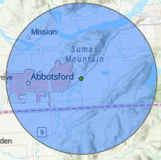
Given that Abbotsford is the largest city in British Columbia by area, the buffer layer created for the major cities was based on the Abbotsford municipality such that the buffer encompassed the entirety of the urban development boundary to be conservative. A buffer of 15 km ensured that the Abbotsford boundary was essentially entirely captured, as pictured below.
The buffered cities layer was then appended to the buffered roads layer and assigned a value of zero given wetlands cannot be developed on existing infrastructure.
Figure 6. City of Abbotsford with a 15 kilometer buffer.
Roads
The roads layer was buffered by 40 meters on each side and then merged with the buffered cities layer. Given that wetlands can exist directly adjacent to roads, the buffer for this layer was relatively small compared to other layers. Since this feature was converted to a raster with a resolution of just under 80 meters, a buffer of 40 meters on each side was the minimum size possible for the purposes of this analysis.
Soil
The soil data already utilized a discrete classification system, with V (very poor), P (poor), I (imperfect), M (moderately well), W (well), R (rapid), and E (excessive) classes. These classes of soil drainage were aggregated into 5 numerical classes according to the paper “A multi-Criteria Wetland Suitability Index for Restoration across Ontario’s Mixedwood Plains” (Medland et al., 2020).
Groundwater Level
Shallow groundwater should be prioritized in wetland mitigation plans according to the study “Wetland spatial dynamics and mitigation study: an integrated remote sensing and GIS approach” (Sivakumar et al., 2016). The groundwater level is important because wetlands are characterized by being either permanently or seasonally covered by shallow groundwater in which the water table is at or near the surface to support hydrophytes as the dominating vegetation type (Medland et al., 2020).
Slope
According to the paper, “Guidelines for free water surface wetland design,” the slope of a wetland should be essentially zero in order to ensure an equal water distribution, preserve the stability of the bank, and maximize shallow water foraging habitat for various invertebrates, fish, and birds (Giuseppe et al., 2000). More specifically, “a uniform longitudinal bottom slope from inlet to outlet should range from 0 to 0.5%” (Giuseppe et al., 2000). However, while it is acknowledged that steeper slopes are more vulnerable to erosion, it should be noted that there is no standardized slope value that guarantees stability (Giuseppe et al., 2000). For the purposes of this analysis, we proceeded with the same 3 classes for slope as used in the study “A multi-Criteria Wetland Suitability Index for Restoration across Ontario’s Mixedwood Plains” which corresponds to the study mentioned above having a 0.05% (0.29 degrees) slope as the maximum optimal slope (Medland et al., 2020).
Stream Proximity
This polygon line layer consisted of all the stream channels in BC. Scaling down the stream to fit the suitability criteria was done by deleting selected stream orders that were less than five. This method would leave only the fitter streams which were more suitable for wetland creation. Closer proximity to streams was prioritized and was placed into two buffer zones: 250m and 500 m. Classes were applied to each buffer, valued at 10 and 5 respectively (Medland et al., 2020) and a zero value was applied to the area outside of the 500 m buffer,
Major Water Bodies
A lakes polygon layer was derived from provincial freshwater data and integrated into the soil drainage layer since wetland creation under a lake should be considered undesirable regardless of the soil drainage assigned to that area. This layer thus only required one class, that being zero. In this sense, the major water bodies layer served as a constraint for the analysis, locating areas where wetland cannot be created (Medland et al., 2020).
Manual Weighted Overlay
Equal weighted
Original 0-10 classes were multiplied by 16.67 (100 / 6) to ensure the scale of the equal weight and weighted versions were the same. Each input was subsequently added together using the Raster Calculator tool and optimal areas were isolated via the Locate Regions tool. The equal-weighted, overlay serves as a sensitivity analysis.
| Input | Reclassification |
| Agricultural Land Reserves | MCE * 21.8 % |
| Built-up | MCE * 12.3 % |
| Soil drainage | MCE * 48.2 % |
| Groundwater level | MCE * 4.7 % |
| Slope | MCE * 2.8 % |
| Stream proximity | MCE * 10.2 % |
Weighted
Original 0-10 classes were multiplied by respective weights from the paper “A multi-Criteria Wetland Suitability Index for Restoration across Ontario’s Mixedwood Plains” such that relative weights were maintained for the raster overlay (Medland et al., 2020). Each input was subsequently added together using the Raster Calculator tool and optimal areas were isolated via the Locate Regions tool.
| Input | Reclassification |
| Agricultural Land Reserves | MCE * 16.67 % |
| Built-up | MCE * 16.67 % |
| Soil drainage | MCE * 16.67 % |
| Groundwater level | MCE * 16.67 % |
| Slope | MCE * 16.67 % |
| Stream proximity | MCE * 16.67 % |
ModelBuilder was used to aggregate the two outputs and delineate areas of overlap. Areas of overlap between the weighted and unweighted overlay rasters were prioritized as high suitability for wetland compensation given the higher certainty associated in areas in which both models agree. We found that the overlapped area alone was not sufficient to compensate for the wetland being lost (513.6 km²), therefore, we also added some weighted optimal areas, giving priority to areas closest in proximity to the overlapped locations.