Unfortunately, the only time I’ve ever visited Singapore was in transit on return to Australia from Malaysia. However, a fellow graduate resident, Joe Daniels at Green College is a “Singapore-aficionada”.

So I asked Joe, “What’s the traffic like in Singapore?” His replied that he was involved in a traffic jam when he first arrived, but didn’t face another problem in over a year there. His overall assessment was that Singapore had “one of the best systems I have experienced and one of the easiest places to travel around”.

These comments are consistent with Singapore recently being among ten cities honoured for their efforts to manage traffic congestion at the Inaugural C40 & Siemens City Climate Leadership Awards (London, Sept 2013).

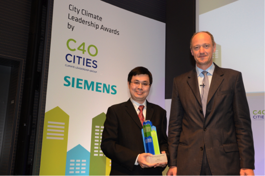
City Climate Leadership Awards (2013)

But it wasn’t always this way. Let’s take a walk back into history thirty years….

Singapore’s traffic dilemma

 The problem of traffic congestion is a vexing one for individuals, employers, city planners and policymakers alike in most major cities globally. For Singapore, it was a particularly pressing one. Singapore had transitioned as a strong emerging economy in the 1970s, with impressive economic growth and increasing wealth and urbanization of Singaporeans.

As result of this spectacular growth was the presence of an increasing amount of vehicles on the road. However, the geographic land characteristics of Singapore were providing a finite constraint. In 1975, there were three million people living in a land area of 633km², with an income per capita higher then many Asian economies.

Something had to be done. Demand on the limited resource base of Singapore was reaching severity and the climate of Singapore is humid and hot, which further increased demand for private, air-conditioned travel.  We have learnt that building more roads is not a conditional solution to road congestion as more cars fill the roads. However, in the confined land space context, building new roads was not an option for the nation. Therefore, Singapore had to look to policies to reduce kilometres driven and cars on the road.

The ALS and ERP

The Area Licensing Scheme (ALS) was introduced in 1975 and was considered “a bold move” as the first congestion pricing program internationally (Phang and Toh, 2004).

It set a price for driving in a ‘Restricted Zone’, which was located in the most congested part of the city. If a car or taxi entered the zone during the peak morning period (7.30-9.30am) they had to purchase a supplementary license sticker for their car. The stickers cost US$4.87 (daily) or US$99.68 (monthly) (2006 prices) and were checked by officials at the 22 points of entry to the Zone (Palgrave, 2006). In addition, public garages in the zone had their average fees doubled. The policy covered cars and taxi’s, but exempted cars with four or greater occupants.

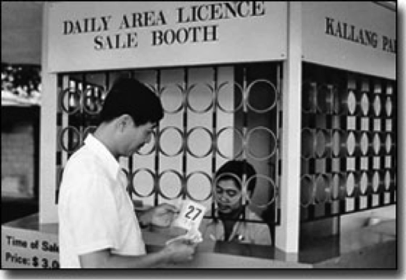
Buying a daily area license at the license sale booth, 1975 (WorldBank)

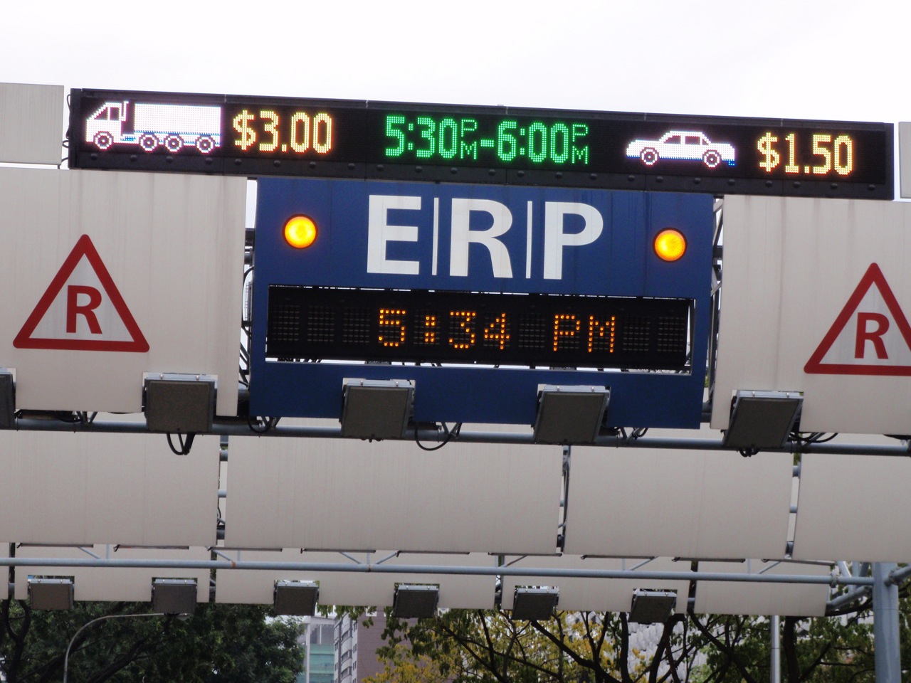
The manual toll system was replaced in 1998 with Electronic Road Pricing (ERP). The tolls were based on size of the vehicle, route taken as well as the time of day.

It was seen as a superior system as it replaced the labor intensive ALS, which had a complicated breadth of licences (16 types), as well as having problems with illegal switching (Phang and Toh, 2004).  In addition, the unlimited number of entries into restricted zone under-penalised contributions to congestion and made it difficult to equate Marginal Social Benefit with Marginal Social Cost (Phang and Toh, 2004).

Why price the roads?

The theory behind pricing road use has been extensively documented. Roads are a public good and a marginal user of the road consider their own private costs whilst ignoring the social cost of using the road.

Pricing the roads in Singapore is an example of a Pigouvian tax. The argument for a Pigouvian tax is as follows; increase the individual cost of usage by an amount that is equal to the externalities imposed by an individual driver. It is judged to be an effective response to tax the externality as drivers are more sensitive to money than the value of time.

Distributional effects on Singaporeans

Several criticisms have emerged in response to the ALS and ERP. To discourage driving, the price had to be set high initially to see a significant and immediate reduction. Phang and Toh (2004) stated that prices were considered to be above the optimal rate as the original target was for 25-35% reduction, whereas the initial reduction was as high as 45%. This has the effect of restricting driving in the zone to those with high incomes only.

The Government responded to this equity issue by ensuring there was adequate public transportation alternatives and additional parking outside the perimeter of the zone (Palgrave, 2008).

Lanier Parking Solutions

Effectiveness

Palgrave (2008) reported “the effects of the ALS were immediate and dramatic, far exceeding expectations”.

Commuters responded in a number of ways to the ALS. Responses included (Palgrave, 2008):

• Car-pooling: the number of cars with four or more occupants increased by 60%
• Public transport: for people who commuted into the Restricted Zone to work and who owned cars, the percentage who chose to ride the public buses rose from 33% to 46%.
• Time substitution: other commuters chose to enter the Restricted Zone before 7.30am. The percentage of car trips before 7.30am rose from 27% to 40% for drivers, and from 17% to 28% for passengers.

Palgrave (2008) stated that the nature and flexibility of these responses meant that pricing remains the least-cost strategy for reducing congestion (Palgrave, 2008).

Phang and Toh (2004) take another angle. They conclude that the success of the “draconian measures” can be attributed in part to the small size geographically of Singapore. This meant the grid remains largely insulated from non-domestic motorists. In addition, the authors state that the necessity of the situation resulted in unwavering government commitment. Furthermore, Phang and Toh (2004) attributed its success to a population that is characterized by “obedient, law-abiding citizenry”.

In relation to the ERP, Xie and Olszewski (2005) reported that there was a drop of 15% in inbound traffic, even though the rates were not as high as with the previous system. Per trip charging was attributable to this decrease. Phang and Toh (2004) stated that moved road pricing in Singapore much closer to optimal pricing.

The difference between the costs and revenue of the system are remarkable. Phang and Toh (2004) stated that what is undeniable is that the alleviation of traffic congestion has been achieved at minimal capital and operating costs. Reports have estimated that revenues from the pricing system were, on average, S$80million per year, with annual operating costs of S$16million and an initial capital outlay for the ERP of S$197million (Lincoln Institute of Land Policy, 2011). However, it is not clear where this revenue went.

The other side of the coin

Did the congestion pricing just move the problem elsewhere? Phang and Toh (2004) argued that although it cut down vehicular traffic volume in the Restricted Zone, it merely shifted the crowding in time and place.  People shifted their travel time to immediately before and after the restricted times and peak hour traffic was diverted to “new escape corridors” (Phang and Toh, 2004).

Conclusion

This very brief look at congestion pricing in Singapore has shown that time-variable pricing of roads can be an effective way to aid congestion problems.

However in this case, key factors specific to the Singapore context, such as size and urgency, were also part of the answer. Also successes in restricted zones must be weighed against the effects of the shifting of congestion.

It must be noted that the trajectory of only one particular policy was focused on in this blog. However, there are additional policies, such as certificate of entitlement fees and quotas, that have also contributed to reduced congestion in Singapore.

References

Elvik, R and Ramjerdi, F (2014) ‘A comparative analysis of the effects of economic policy instruments in promoting environmentally sustainable transport”, Transport Policy, Vol. 33, May 2013.

Lincoln Institute of Land Policy, (2011), Climate Change and Land Policy, [Puritan Press Inc., New Hampshire]

Olszewski, P and Xie, L., (2005) ‘Modeling the effects of road pricing on traffic in Singapore’, Transportation Research Part A.

Phang, Sock-Yong and Toh, Rex (2004), ‘Road Congestion Pricing in Singapore: 1975 to 2003’, Transportation Journal, Vol. 43, No.2.

WorldBank, ‘Relieving Traffic congestion ; the Singapore area licence scheme, 1975’, Available online at http://web.worldbank.org/WBSITE/EXTERNAL/EXTABOUTUS/EXTARCHIVES/0,,contentMDK:21029453~pagePK:36726~piPK:437378~theSitePK:29506,00.html

What is the Southern Bluefin Tuna?

The Southern Bluefin is a highly migratory, fast swimming fish that live in open seas. As a result they support several international fisheries.

Ocean Tracks, CSIRO

They begin their life in warmer water in spawning grounds between Australia and Java. From there, juvenile fish leave the spawning grounds, and move south during summer along the Western Australian coastline towards the Great Australian Bight. They also travel west towards South Africa through the Indian Ocean (Welburn, 2011, Mori, Katsukawa et al, 2001).

The Southern Bluefin Tuna are fished by high seas long-line vessels and purse seine. Upon catching (between 13 and 25kg), the fish are towed back alive to “static growth pontoons” off Port Lincoln in South Australia. After six months of being grown out, they are harvested and exported, mainly to Japan (AFMA). The overwhelming majority of the fish is sold in the Japanese sashimi market (The Conversation, 2013).

Bureau of Rural Sciences, Australia

The problem

Southern Bluefin Tuna have historically been heavily fished since the 1950s, which has resulted in decline of mature fish as well as annual catch falls. The over-fishing has been to levels that are above the average maximum sustainable yield.

The International Union for Conservation of Nature (IUCN) has a ‘red list’ that categorizes species according to their vulnerability of extinction (Welburn, 2011). The Southern Bluefin tuna has been red listed as a ‘critically endangered species’ due to its rapid decline in quantity (Punt, 2008, in Welburn).

Policy reaction

A voluntary mechanism to limit catch was introduced by Australia, NZ and Japan from 1985. In 1993, there was a move to a more formal management mechanism, with the creation of the Commission for the Conservation of Southern Bluefin Tuna (hereafter CCCBST), headquartered in Canberra.

The Republic of Korea, Indonesia and Taiwan joined the original three in 2001, 2008 and 2002 respectively and the Philippines, South Africa and the European Community were formally accepted as “Cooperating Non-Members in 2004, 2006 and 2006 respectively (CCSBT).

Policy mechanism

Catch for the Southern Bluefin Tuna is regulated via two mechanisms, a global total allowable catch (TAC) as well as individual country-specific transferable quotas (ITQ) set by the CCSBT.

In Australia, the ITQs are allocated as Statutory Fishing Rights. The Australian Fisheries Management Authority (hereafter AFMA) determines a TAC for the Australian domestic fishery, which is based on the allocation from the CCSBT. A Statutory Fishing Right then entitles the holder to receive an equal portion of the TAC set by the AFMA (AFMA, 2012).

A formal rebuilding management regime was adopted in 2011 in response to significant under-reporting discovered. The 2011 management procedure (harvest strategy) aimed to guide recovery of biological stock to 20% of unfinished biomass by 2035 (FRDC, 2012).

The “management procedure” provided guidance for the CCSBT to set global TAC as well as to provide the “fishing industry with stability in the level of catch over a set period of time” (DAFF, 2012). The TAC can be updated based on monitoring data, according to the following parameters:

• set for three-year periods
• built on a 70% probability of rebuilding the stock to the interim target point of 20% of the original spawning stock biomass by 2035
• the minimum TAC change is 100 tonnes
• the maximum TAC change is 3,000 tonnes.

 The FRDC reported that the CCBST set the global TAC for 9,449t (2010), of which Australia had the largest quota of 5,265t (2010). The Australian Fisheries Management Authority reported that approximately 96% of Australia’s quota is caught by five purse seine vessels.

CCBST, 2012

Monitoring and surveillance

The CCSBT has several monitoring, control and surveillance schemes including:

• Catch Documentation Scheme (2010): tracks and validates legitimate flow from catch to point of sale on domestic or export markets
• Monitoring of SBT Trans-shipments at Sea (2009): applied to long-line vessels with freezing capacity.
• Approved Vessels and Farms: not allowed to land or trade SBT caught by those not on the list
• List of Illegal, Unreported and Unregulated (IUU) Fishing Activities (2013): identify vessels engaging in IUU each year
• Vessel Monitoring (2008): Members and co-operating non-members required to adopt and implement satellite vessel monitoring systems.
• Action plan: to build cooperation in supporting management and conservation measures. CCBST has advised if cooperation is not forthcoming, measures including trade restrictive measures, may be taken against them.

A separate by-catch and discards work-plan has also been developed (AFMA). In relation to boat numbers, although the number of active global vessels catching SBT is not available, the most recent estimates cite approximately 1,296 vessels in 2010 (FRDC, 2012). In Australia in 2010, six purse-seine vessels and 18 long-line vessels caught SBT (FRDC, 2012).

Potential advantages and disadvantages

1)    TAC size

The most recent figures for 2011/12 provided by the AFMA, recorded:

• Agreed Australian TAC: 4,528t
• Reduced TACL 4,509t (because overfished in previous year)
• Catch: 4,543t
• GVP: $40,503,000
• Farm gate value: AU$150million

The catch of 4,543t can be compared to a 21,000t TAC, which was implemented, but not binding, by the Australian government in 1983 (Coombs, 1997). This represents major progress in responding to the reduced Southern Bluefin stock. In addition, the TAC can contract and expand, which produces an incentive to increase the overall stock to increase individual share.

However, is it enough? As discussed above, quotas are set for three years to provide stability for fisherman. They can also increase, which they have, which has brought fierce criticism from environmental groups. Greenpeace (2013) slammed the three consecutive years of increase in quotas and called for “zero catch” as “the only way to ensure survival of a species decimated by overfishing”.

 “The Southern Bluefin fishery has been a case study in mismanagement and this new announcement continues to play Russian roulette with the survival of an entire species.”

Nathaniel Pelle, Greenpeace Oceans Campaigner

 “Current stock assessments show that this is already a fishery in collapse. The simple truth is we need to leave the Southern Bluefin tuna well alone for a while so that stocks can recover as quickly as possible.”

 Pam Allen, Australian Marine Conservation Society campaigner

2)    Suitability of ITQs: price and fleet response

 The use of ITQs suits Southern Bluefin fisheries for a number of reasons, as outlined by Coombs (1997):

• They are a long-lived species with small annual variations in parental stocks
• Market outlets were relatively few and well defined, which may reduce black market sales and the costs of enforcement.

In response to early ITQ’s, the average price of Southern Bluefin Tuna increased by more than double. In addition, Coombs (1997) reported that the system allowed Australian fisher’s to maximize the value of their catches “by concentrating on larger fish rather than maximizing the total amount of their catch (as is the incentive with aggregate quota schemes).

The ITQ changed the structure of the Australia fleet as fishermen had two choices: sell quota and exit the market, or buy additional quota. Many New South Wales and Western Australian fishermen exited the market and those remaining purchased additional quota and subsequently had to increase the scale of their respective operations (Coombs, 1997). However, as Coombs (1997) explained, although the ITQ reduced the amount of Southern Bluefin caught and increased efficiency of the fleet, they did not succeed in restoring parental biomass to desired levels. 

3)    Global agreement

For a highly migratory species, it is difficult to enforce global participation to reduce overfishing. The Southern Bluefin Tuna TAC has been an example of international cooperation and enforcement.

However, it is also due to the global nature of the system that causes problems. The Conversation (2013) argued that there is often decision paralysis and status quo management because management is via international agreements on quotas. They noted that this management system “can be slow to respond to problems such as low numbers, leaving the population ill-equipped to deal with the vagaries of juvenile survival” (The Conversation, 2013).

4)    Illegal fishing

As discussed above, there is significant enforcement and monitoring in place, that far outstrips many other fish policy initiatives. However, IIU continues to be an issue with reports of declines in mean lengths of Southern Bluefin in spawning grounds. This has been an indicator of Indonesian vessels fishing below the spawning grounds south (AFMA, 2013) and the issue is currently being investigated further. 

Current state

The Conversation (2013) reported that the current best scientific advice is that mature biomass is between 3-8% of the tuna’s un-fished level. This is well below sustainable levels. Supporting this, the stock assessment completed by the CCSBT in 2011 suggested that the spawning biomass is well below the level that could produce maximum sustainable yield (AFMA). The FRDC (2012) reported that measureable improvements in spawning stock are yet to be detected and the stock status remains “OVERFISHED”.

However, the AFMA reported that there is a positive outlook for stock based on the 2011 assessment, which include a continued reduction in total reported global catch. In addition, the current mortality has reduced below F_msy (maximum rate of fishing mortality: proportion of fish stock caught and removed by fishing) and stock is expected to increase at current catch levels (AFMA, 2012).

References

Australian Fisheries Management Authority (2012), ‘SBTF at a glance’, Available online at http://www.afma.gov.au/managing-our-fisheries/fisheries-a-to-z-index/southern-bluefin-tuna/at-a-glance/

Commission for the Conversation of Southern Bluefin Tuna, ‘Origins of the Convention’, Available online at http://www.ccsbt.org/site/about_commission.php

Coombs, J., (1997), ‘ Individual Transferable Quotas in Fisheries’, Available online at http://personal.colby.edu/personal/t/thtieten/itqs-aus.html

Department of Agriculture, Forestry and Fisheries, (2012), ‘Commission for the Conversation of Southern Bluefin Tuna’, Available online at http://www.daff.gov.au/fisheries/international/ccsbt

Fisheries Research and Development Corporation, (2012), ‘Southern Bluefin Tuna’, Available online at http://www.fish.gov.au/reports/finfish/tuna_and_billfish/Pages/southern_bluefin_tuna.aspx

Greenpeace Australia Pacific, (2013), ‘Increased quotas will decimate critically endangered southern Bluefin tuna’, Available online at http://www.greenpeace.org/australia/en/mediacentre/media-releases/oceans/Increased-quotas-will-decimate-critically-endangered-southern-bluefin-tuna—Environment-groups-call-for-zero-catch-4/

The Conversation, (2013), ‘Australian endangered species: Southern Bluefin Tuna’, Available online at http://theconversation.com/australian-endangered-species-southern-bluefin-tuna-11636

Welburn, N., (2011), ‘Reversing the decline of the Southern Bluefin Tuna. Are Marine Protected Areas the Answer?’, Bangor University. Available online at https://www.academia.edu/2343330/Reversing_the_decline_of_the_southern_bluefin_tuna._Are_marine_protected_areas_the_answer

The In’s and Out’s of Australia’s Carbon Policy

<<This post was created as part of a course requirement for ‘Environmental Economics and Policy’ >>

Carbon policy is inherently complex, uncertain and highly political. Australia is no exception to the case, and may in fact have taken it to another level completely, being the first nation to abolish a carbon tax after only one year in administration.

‘It’s official, Australia has a carbon tax’ (The Australian, November 08, 2011)

…but less than two years later…

‘Tony Abbott locks in death of carbon tax’ (The Australian, August 16, 2013)

In September 2013, Australia heralded in their 28th Prime Minister, Coalition Leader Tony Abbott. Upon winning the Federal election convincingly, Abbott’s first order of business, as promised, was to repeal the Carbon Tax. The Coalition had built their election platform on the disbandment of the Clean Energy Act 2011 in favour of a ‘Direct Action Plan’, which looks to incentivize industry directly to reduce emissions. Thus, whilst many countries are working to introduce, iron out and implement carbon taxes, Abbott is committed to push through legislation to dismantle ours.

Sydney Morning Herald (2013)

So what is it that Abbott is repealing? It is important to first understand our current Carbon Policy, its coverage as well as distributional effects. We can then begin to compare Australia’s policy to the rest of the world, as well as to the ‘Direct Action Plan’ that Abbott is suggesting to replace it.

Clean Energy Act 2011

In 2011, a package of carbon pricing bills was passed through the House of Representatives. The central tenet of the act, the Carbon Pricing Mechanism (CPM), which took effect on July 2012, introduced an emissions trading scheme that put a price on Australia’s carbon emissions.

Julia Gillard, Labour Prime Minister, coined the term ‘carbon pricing mechanism’ when communicating the party’s carbon policy. This was in response to several announcements as part of her winning election platform where she promised she would not introduce a ‘carbon tax’.  However, many have argued that there was no practical difference between a fixed carbon price and a carbon tax, as they both drive up the cost of energy to bring about a reduction in energy use (Professor Michael Dirkis, ABC, 2014). The label of the policy became a point of contention and Gillard was consistently caught up in definitional debates. Gillard admitted recently that “her decision not to argue against a fixed carbon price being labelled a “tax” hurt her terribly politically” (ABC, 2014).

The CPM was to be introduced in two phases, with a fixed phase, beginning in 2012 to be following by a flexible price in 2015. Initially, the price of carbon units would be $AUD23.00 (2012), $AUD24.15 (2013), and $25.40 (2014), with a floor price of $15.00. During this period, there was to be no limit on the amount of permits able to be purchased. The second phase was to be characterized by a cap-and-trade system, where the Government would set caps on the number of units to be issued each year (Minter Ellison, 2012). Supply and demand forces would interact to determine the price paid for available carbon permits.

Coverage

In 2011, Australia’s emissions profile looked something like this:

Climate Change Authority, 2011

So who was in and who was out? In regards to coverage, Australia’s Clean Energy Regulator (2014) stated:

“Generally, if a facility meets or exceeds the threshold of covered emissions with a carbon dioxide equivalence (CO2-e) of 25 000 tonnes in a financial year, the person responsible for such a facility will be liable under the carbon pricing mechanism”.

However, not all of the sectors in the chart above were covered as part of the carbon tax threshold.  Those industries covered (if above the annual threshold) included:

• Stationary energy (e.g. Electricity generation)
• Industrial Processing (e.g. Aluminum smelting)
• Fugitive Emissions (other than from decommissioned coal mines) (e.g. Emissions from extraction of coal, oil and natural gas)
• Emissions from landfill waste and waste water treatment (legacy waste exempted).

Emissions not covered by the CPM were:

• Agriculture
• Land use, land use change and forestry
• Fugitive emissions from decommissioned mines
• Conventional road transport
• Entities covered in CPM but fall below threshold

ClimateChange.Gov.Au, 2011

It was believed that 400-500 liable entities were covered under the scheme (between 50 and 60 per cent of Australia’s emissions), with another 4-7% via equivalent carbon pricing (Clean Energy Future, 2011). The equivalent pricing was to cover remaining sectors (domestic aviation, marine and rail transport) through separate legislation. This coverage was reported to be comprehensive and is reasonable compared to other countries (i.e. Norway’s tax covers approximately 65% of emissions).

Distributional Impacts

As the worst carbon-emitting nation per capita in the OECD, many saw the Clean Energy Act 2011 as a crucial first step in Australia playing a role in global climate change action. Andrew Hewett, Oxfam Australia Executive Director (2011) stated that “Australia has until now failed to contribute its fair share to global efforts to fight climate change. Passing this legislation is a crucial step in playing climate catch-up”.

However, the passing of the bill was met with mixed responses from Australian industries and consumers, as people were fearful of broad economic as well as individual distributional impacts. A flurry of discontent ensued due to expectations of flow on to consumers of businesses passing through increased costs through the supply chain. Also, as a resource-rich, net exporting country, many were concerned that the carbon tax would negatively affect our industry competitiveness on the global stage.

Australian Conversation Foundation, 2011

The Conversation, 2011

Distribution of the tax burden is an important policy consideration, for reasons of equity and political feasibility (Goulder and Schein, 2013). In response to regressive distributional effects, the Government responded by confirming that revenue from the carbon tax would be distributed to businesses and households in the form of compensation. Tax cuts, increases in allowances, payments and benefits were introduced to offset the average rise in household costs of $9.90 per week. Approximately 50 per cent of scheme revenue generate was to be used to compensate households and industry, however it was not revenue neutral as per BC’s Carbon Tax. Industry assistance mechanisms (Deloitte, 2011) included:

• Jobs and Competitiveness Program for Emission-Intensive Trade-Exposed Assistances. $9.2billion over three years to 2015 in form of free permits and grants to increase energy efficiently.
• Manufacturing Industries Clean Technology Program – $1.2billion to assist manufacturing industries.
• Coal Sector Jobs Package – $1.3billion over six years to manage transitional impact.
• Energy Security fund – Assist electricity sector deal of free permits and cash of $5.5b over six years as well as pay for closure of very high emitting coal-fired generators by 2020.

Enter Tony Abbott

Move forward one year in the CPM, July 2013. Results so far are mixed. One side reports that emissions from electricity are at a ten-year low, renewable power generation has increased by almost 30% and the CPM had “clearly not been the wrecking ball it was dubbed” (Huffington Post, 2013). On the other hand, Economist Alex Robson of Griffith University, stated the main effect of Australia’s carbon tax has been to significantly increase electricity prices for households and businesses, with no reduction in CO₂ emissions (Alex Robson, 2014).

Enter Toby Abbott and the argument for pro-business and “common sense action”.  Arguing on the limited effect of the tax on emissions, problems with artificial price setting and anti-competitiveness, the Coalition set out to “clean up the mess of the Carbon Tax imposed by the previous Labor-Greens Government” (Kelly O’Dwyer, 2013). The proposed ‘Direct Action Plan’ concentrates on funding private industrial financed initiatives through taxpayer money to reduce emissions as well as sequestration of atmospheric C0₂ (Lubcke, 2013).

Department of the Environment, 2013

The plan may be more palatable for industry and pragmatic for decision-makers. However, it still infers an implicit carbon price that may actually be higher for Australian taxpayers and may encourage free riders.

Maybe Australia won’t throw out our “baby with the bathwater” (Kelly Rigg, 2013) as the latest update (6 March, 2014) finds:

“Prime Minister Tony Abbott’s plan to scrap Australia’s carbon tax regime took a hit this week after the Senate failed to pass legislation to dismantle the independent Climate Change Authority.

Christine Milne, leader of the Green party in the Senate, said, “The Greens, with the balance of power in the Senate, saved the Climate Change Authority … because we know it’s more important than ever that Australia doesn’t succumb to inaction on climate change…”

(Taxnews.com, 2014)

Watch this space.

Memories of drought are unsettling. Devastatingly unsettling.

The decade spanning 2000-2010 was the last straw for so many Australian families and communities who were forced to close the door on their torrid love affair with the land. The relentless and monotonous dry months took their toll on those nearest and dearest to me and across the country.

Tonight, in 2014, on the other side of the world, my heart goes out to those at home who are once again in such a desperate situation. I see Twitter posts of rain and hope that it doesn’t stop anytime soon.

Thankfully, details of drought relief packages are being released. Barnaby Joyce, Australian Agriculture Minister, is apparently putting ‘the finishing touches on a drought support package’ (ABC, 2014) as I write this. The National Farmer’s Federation Drought Relief Package package includes improving access to income support, low interest loans, water infrastructure grants, farm-labour wage assistance and farm advisory grants. I urge anyone interested to read their packages of immediate drought relief measures.  ‘Farmer’s across the country need support now’, Brent Finlay, NFF President stated. Support in the form of drought assistance loans is needed right now to get through this acutely tough time that is destroying whole communities.

However, the word ‘support’ and ‘relief’ conjure up short-term fixes, a ‘leg-up’, a prop, a brace.

In the longer-term,  we need to start thinking about structured drought policy. Creation and implementation of such a policy, however, is not going to be an easy road. Although drought has been a significant and recurring part of our nation’s history, our climate is changing, and with it, increased severity and frequency of such disasters. We have to start thinking about drought policy in this context.

This, however, is difficult when our own Prime Minister states offhandedly that ‘there have always been tough times and lush times’ and continues to dismiss the link between drought and climate change. Relief packages are required when these ‘bad times’ (Abbott, really?) hit, no doubt, but there has to be comprehensive thinking and work done that is conscious of longer-term climatic challenges. But with a Prime Minister that doesn’t see the threats that come with changing mean variable temperatures, I can see that investment into future agricultural and drought policy will be limited. Tony, how do you think your grand plan for a Northern Australian ‘food bowl’ will succeed without taking into account the likelihood of drought occurring more severely and frequently in the coming century?

Brent Finlay (NFF, 2014) also advocates for long term drought policy solutions, however notes the problems inherent in timing. He notes, ‘when there’s not a drought on, it’s difficult for preparedness to remain a top priority for Government, as we have seen in recent years’. While current needs of farmers and communities are being addressed by relief packages, going forward we need to focus on significant inquiry, even if the drought ‘breaks’. I do not say this to detract from the priority of helping those in need now, particularly those that had not seen rain for two years until today. However, as noted by West Australian Nationals leader Terry Redman “The significant shift is moving from crisis management to risk management and that’s the policy setting shift.” I really hope it does.

What should be included in a longer-term strategy for drought management? Investment in water infrastructure? Input subsidies? Adaptation measures? According to the OECD’s Agricultural Policy Monitoring and Evaluation Report 2013, Australian farmer’s continue to have some of the lowest producer support mechanisms in place. Although this is troubling, pure support in the fashion akin to other countries is not necessarily the solution. Distortionary input subsidies may certainly not be the answer, but we need to at least start to begin to analyse potential policy mechanisms.

A comprehensive review in 2008 was performed that looked at the future of Australia’s climate and the types of drought measures in place. However, the response from government was inconsequential and nothing widespread was been put in place.

Planning for drought cannot be left to times of extreme drought.

Let me begin by stating that this piece is not in support of Abbott’s decision regarding AusAID. His intentions were clear; he simply does not see development aid as a priority relative to other portfolios. If he did, he would have used the opportunity to acknowledge that the current system is not working and to find ways to make it more effective.

Rather then focusing on Abbott’s decision, this blog aims to cut through the polarising nature of the debate to encourage improvements to our current development funding processes.

—————————————

Less than 48 hours out from the Australian Federal Election this year, the conservative Opposition announced that they planned to slash the growth rate of foreign aid spending by $4.5billion over four years. Two days later, this same party won the election, ascending Tony Abbott to the seat of Prime Minister of Australia.

The Australian

The announcement of foreign aid cuts triggered backlash and anger through many sects of Australian communities. In addition to his cries to “stop the boats”, Prime Minister Abbott emblazoned himself as an infrastructure leader who would “put bulldozers on the ground and cranes into our skies”. Disgruntled Former Foreign Affairs Minister, Bob Carr, declared that Australian aid spending (0.37 per cent of national income) was “in our interests” and that “Australian security is served by an effectively delivered foreign aid program” (Australian Network News, 2013). Were we putting ourselves at risk by reducing our foreign aid balance?

Abbott’s move to direct funding towards infrastructure for Australian cities and Carr’s subsequent comments got me thinking more broadly about why Government’s around the world fund foreign aid and if the model is successful for those it intends to aid. Julie Bishop, the new Foreign Minister, made her first major statement on aid in November 2013 that AusAID was being abolished and its functions merged with the Department of Foreign Affairs and Trade. It is being returned to the foreign ministry, with Abbott citing a need for greater alignment between “the aid and diplomatic arms of Australia’s international policy agenda”. Strategic intent is claimed to be at the centre of government funding of aid, with foreign aid programs “always bedeviled by conflicting national foreign policy objectives” (Creighton, 2013).

Is aid purely strategically pragmatic, fueled by emblazoned security concerns? Is it merely a way of privileged nations to symbol their wealth or ascend their guilt? If aid is designed with such notions in mind, how can the resulting programs that they fund be effective, transparent, impactful and responsive to the real needs and voices of often-distant communities?

—————————————

The aim of this piece is not to take a side on whether government aid funding cuts are right or wrong, rather the objective is to show the importance of asking the right questions before condemning an action. My initial response to Abbott’s announcement, following a brief squirm of resentment, was the desire to understand the current effectiveness of aid that is funded by the Australian Government. If the current program of aid is not – for lack of a better word – aiding developing communities, why should it continue to grow?

Exclusively measuring the amount of money delivered to such programs is, in my mind, a very rudimentary way of evaluating the effectiveness of aid. Following my coursework focused upon the Monitoring and Evaluation of Timely Responses (METR) for development, I find evaluations of aid that focus purely on inputs and outputs, with no attention given to the intended and unintended impacts of programs, negligible. We should be asking what the intended impact is, the long-term objective, and if the billions of dollars that go into development aid are effective against them. Are we wasting our aid dollars on programs that aren’t working?

Lowy Interpreter

—————————————

AusAID was tasked with a complex undertaking. An Audit Report of AusAID’s management of the expanding aid program (2010) stated that the scaling up of Australian aid and the impetus to change how aid is delivered amplified key challenges. A key finding of the audit was that continued improvement in the monitoring and evaluation of aid is required to if AusAID is to remain in a good position to meet the challenges of the coming years (ANAO Audit Report, 2010).

For every example of a successful development program, I can only guess the disproportionally high degree of failures. An article focused on AusAID’s failure of commitment to human rights in Cambodia (Macdonald, 2013) is one such example. The article opens in a poignant manner with the author openly stating that a Cambodian infrastructure development project has resulted in the displacement and violation of people’s land rights. He notes that this may not be surprising in a country that is recognised for its entrenched poverty, financial opportunism and government heavy handedness. What is surprising, however, he notes, is when these projects are “financed and managed by the organisation’s whose stated purposes are to work to improve the lives of world’s poorest and most vulnerable” (MacDonald, 2013).

Ausaid

AusAID provides 15 per cent of the financing for the Railway Rehabilitation Project in Cambodia as part of its “Australian-Cambodia Joint Aid Program Strategy 2010-2015”. A project that aimed to link Cambodians with each other and with external markets has been plagued by inadequate consultation, compensation and displacement of local people. Those relocated have inadequate access to basic services and employment. A report published by Aid/Watch notes that the obsession with ‘economic development’, over human development, including the privatization agenda, are specifically troubling – “the project has been unable to articulate in any way how it will effectively reduce poverty” (AidWatch, 2012). Although AusAID may have had good intentions in entering the Cambodian project, such intentions are inadequate, and “ignorance is cold comfort to the people whose lives have been destroyed” (AidWatch, 2012).

The Cambodian Daily

This example is only one of many of the projects that Australian aid has funded that are in line with our ‘strategic interests’. Although I do not condone the actions of Abbott in cutting the budget, I do embolden our leaders to implement transparent and accountable monitoring and evaluation procedures that are context-specific and put the beneficiary at the heart of the development agenda. I acknowledge that measuring the effectiveness of development aid is inherently complex and difficult, particularly when there exists uncertainties about intended objectives and the isolation of causal effects. But, that is not an excuse to only measure those hard and fast indicators that are ‘easy’, such as dollars spent or programs funded. Let’s begin by assessing the intervention logic, the design of the program itself and it’s relevance. What are the intended and unintended benefits and costs of the project to the multiple stakeholder groups?

—————————————

Let us rethink how to more appropriately spend development aid by monitoring and evaluating projects in a timely manner and by asking the tougher questions. If Abbott invests money in an independent evaluation house to do so, he will have my attention. Slashing the budget in itself is not a helpful solution to the problem of aid not being effective. 

This week during a post-exam glass-of-wine downtime Ariel and I started chatting about what parts of the MFRE program we were enjoying, what we weren’t and the gaps we saw currently. It turned out to be a really productive conversation that finished with an idea I want to share here with my classmates.

Our program is intensive and we are learning from some remarkable professors. We are busy learning about pricing models, ways to analyze quantitative data and development projects, as well as how to trade in futures markets.

However something is missing. We felt a gap in our understanding of what was happening in the world now. Being able to be informed enough to ask the right questions is fundamentally important to learning, however I feel a little naïve about current movements in research, debate and policy related to agricultural economics.

So we got thinking….

I mentioned to Ariel that this week I was planning on taking a week off from trading and dedicate my blog to a literature review of a recent journal article related to the futures market and trading more generally.

As I spoke, a light bulb went off in both our heads! That is what we are missing. We are simply not reading enough. We briefly paused and thought to ourselves, ‘How the hell am I going to fit time for this into my current schedule?’ Such notions were quickly pushed aside as we realized the huge opportunity we had to gain by simply reading more, understanding the research that was being performed and critiquing what was out there.

So we are setting up a “Reading Group”, that will be trial based for the remainder of Term 1 with hopes of cementing something more formal in Term 2. We hope to invite Professors to share their work with us (I’m looking at you Sumeet) as well as help us to guide us in our reading. In time, we hope to squeeze a little bit of funding from LFS (I’m looking at you Pradip!) to enable us to have coffee and baked goods to aid the discussion! It won’t be compulsory, graded, or intimidating, but it will be exciting, full of learning and hopefully insightful!

Our idea has already been activated by Ariel looking at the seminal ‘How to Understand High Food Prices’ by Christopher L. Gilbert, which appeared in the Journal of Agricultural Economics. We felt it was a good starting base and related to our 501 trading exercise as well as the theoretical content. Hopefully it will wet enough appetites to garner some interest!

In the lab on Tuesday I hope to introduce our idea as well as briefly look at a current journal article. Watch this space because I am still deciding!!

Over the weekend, I was lucky enough to venture outside of Vancouver for the first time since arriving in the Northern Hemisphere. My darling best friend was visiting from Chicago (where she has recently relocated with her husband) and we went on a few adventures! Whilst feeling blessed that the Vancouver sun was shining, we discovered Squamish, rode horses by rivers and through forests, biked around Stanley Park, enjoyed great coffee, aquarium-visited, Wreck-beached and ate a ton of sushi. It made for a memorable and breathtaking weekend and I definitely fell in love with BC a little bit more!

Riding in Squamish

Alice Lake, a Beluga whale and a parrot (breed unknown!)

After taking my mini-break, I felt overwhelmed with the amount to achieve this week. However, I hoped to attempt to implement some of the technical analysis that was shared with us in our trading lab (plus a few other ‘shapes’ I discovered on my own).

—————————————–

To this point, I had primarily based my trading strategy on external information and broader market movements. My aim was to focus upon Live Cattle futures (which I dove into last week for the first time), try and see some trends or signs in the closest futures contract (Oct 2013), and attempt to make some quick profits! It was a little quick and dirty due to time constraints, but hoping the some of the analysis is technically correct!!

This guy’s strategy is a little more fine-tuned than mine!

—————————————–

The graph below shows the daily movement for the October Live Cattle Futures contracts since July. I found three trends to focus my trading decision on this week: the rising wedge, the cup and handle and the ascending triangle. 

——————————-

#1 The Rising Wedge

One ‘shape’ I discovered was the rising wedge from the middle of September to the beginning of October. As seen above, the trendlines are both slanted in an upwards direction and are converging. This wedge is seen to have a bearish pattern and signals that the future is possibly going to head downwards. Research has told me that as the price moves towards the apex of the pattern, the momentum is weakening and a move below the lower trendline is often viewed as a reversal in the upward trend. At the end of September, this happened, with the contract price dropping. Another example of this pattern is seen below.

#2 The Cup and Handle

The second shape was a little more adventurous and  had several components to it that needed to seen in a particular order on order evaluate what the potential signal may be.

Firstly, there should be an upward trend before the formation of the cup. Check. The cup should be nicely rounded, similar to a semi-circle. Mmm, kinda (the reason for this roundedness is that it is a signal of consolidation within a trend – weaker investors start to leave the market and new buyers and more resolute investors stay with the futures contract).

The height of the cup is also important. A traditional pattern should be between 1/3 – 2/3 the size of the previous upward movement. Yep, I can see that has happened in the case of the Oct contract. The height of the cup can also be used as an initial price target when the patten completes by breaking the handle. Lastly, the handle. It completes the pattern and refers to the downward move after the upwards trend on the right side of the cup. The general rule is that the handle retrace’s approximately 1/3 of the gain made in the cup. Most of these signs seemed to have held in the case of the Oct futures contract.

#3 The Ascending Triangle 

Although the first two patterns were interesting to discover, I was looking for something to base this week’s trade on. I found it in the ascending triangle that looked to have developed from the beginning of October. Although, it was not as strong a pattern as the one below, I was going to run with it!

This bullish chart pattern is generally considered to be one that is to continue upwards. It is found within a period of consolidation of an upward trend and once the straight trendline meets the upward one, traders generally enter into long positions. The most common price target to aim for is set equal to the entry price plus the vertical height of the triangle. I decided to buy 6 long contracts on Tuesday morning, hoping for a rise the size of my triangle height!

—————————————–

So far, my ‘analysis’ has paid off and my Oct Live Cattle contracts are up 0.64%. In other news, I shorted 8 Nov Soybeans contracts on the same day (Tuesday morning). Soybean prices had risen on Monday, but I believed this increase would reverse as I predicted solid news to come in about the harvest underway. At the end of the trading week, Nov futures had cemented below its 100-day moving average at $12.865. I was now a richer woman, having made over $14,000 on these contracts!

My portfolio summary as at the 11th of October

—————————————–

In the vein of my blog title, I wanted to end by sharing a little story I heard at the Vancouver aquarium last weekend that was perhaps the most sweet I have ever heard.

Otters hold hands whilst sleeping to stop them drifting apart whilst in slumber. I have known this fact for a while and definitely didn’t need anymore convincing that they were amongst my most favourite of animals. But they were about to get a whole lot cuter!

The trainer at the aquarium told us that a mother otter always keeps her baby on her belly to keep it safe. Before falling asleep she would get some seaweed (kelp) and tie it around herself and then around the baby to create a ‘seaweed seatbelt’ so her baby would never fall off while she rested! I think this is the most adorable story and just had to share that!!!

—————————————–

Happy Thanksgiving everyone!

The following sites helped me perform the analysis above:

Investopedia

Trading Charts