Overview
To answer our three questions we used an MCE (multi-criteria evaluation) to determine the most favourable areas for grizzly movement and settlement. Using different types of land use and land features, both natural and human-made, as our criteria, and using the analytical hierarchical procedure to decide the weightings for use in the weighted sum calculation, this MCE will score the cells in our extent according to how favourable they are for grizzly movement and habitat. We can then highlight areas of interest from the MCE map, such as an extended patch of favourable terrain, which can serve as a potential wildlife corridor (Fig 1).
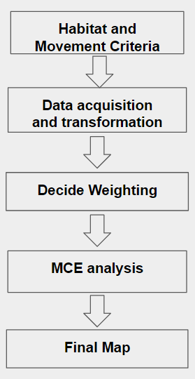
Fig 1. Flow chart of our methodological process to produce a habitat suitability and wildlife corridor analysis of southern B.C. grizzly subpopulations.
DATA TRANSFORMATION AND NORMALIZATION
Combining DEM’s
ArcToolbox -> Data Management Tools -> Raster -> Raster Dataset -> Mosaic To New Raster
Our study area, which contains the majority of southern BC, is composed of grid squares 82M, L, and E and 92O, P, J, I, G, H on the map. To begin working with the data, we needed a base DEM to work with. We started by downloading the DEMs of each grid square and then using the ‘Mosaic to Raster’ function to produce a combined DEM of the region (Fig 2).
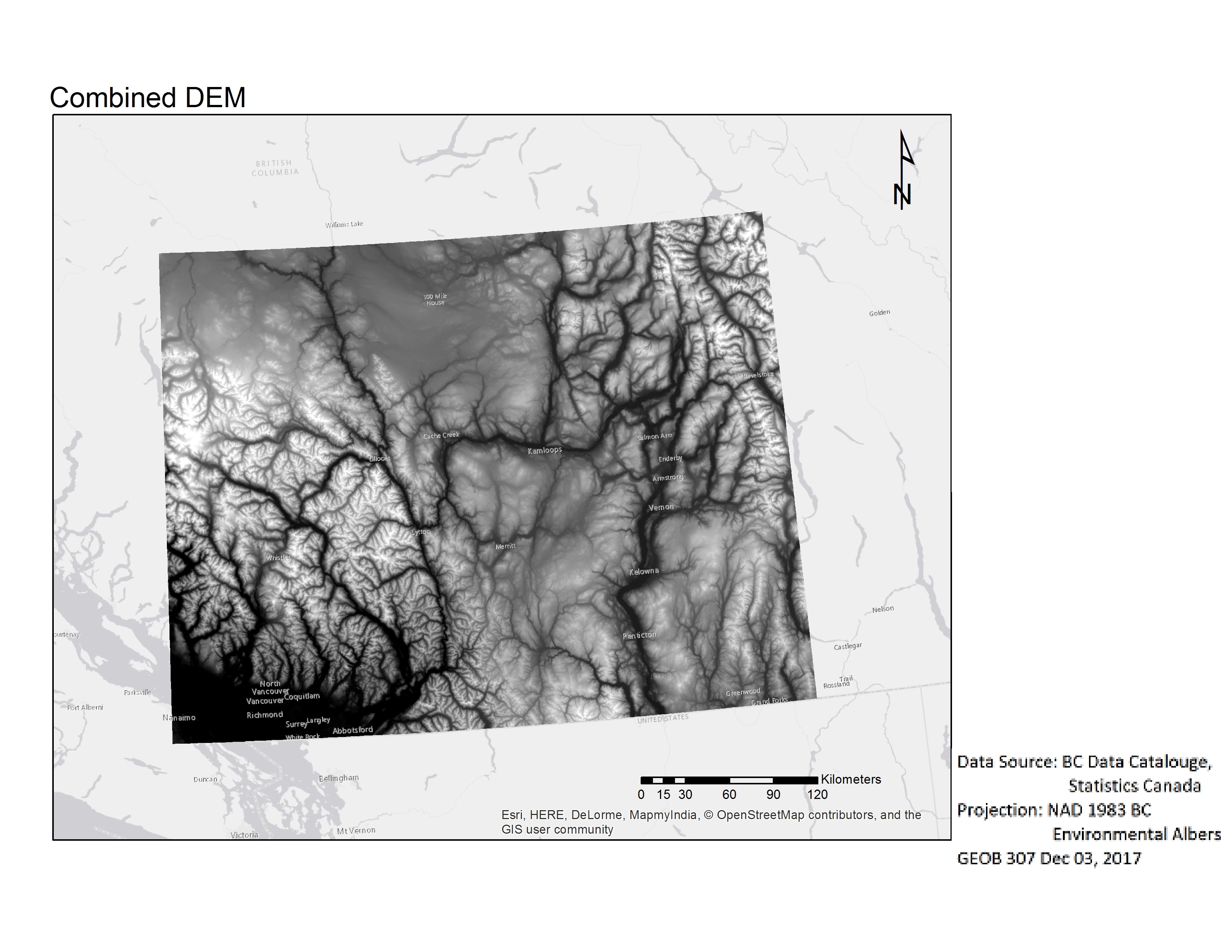
Fig 2. Map of the combined final DEM.
Then to simplify the acquisition of other layers, we created an extent polygon. This would allow us to accomplish two things: creating polygon/polyline layers that matched the extent of our DEM minimizes the amount of clipping transformations we have to apply to any subsequent data retrieved, and minimizing the chances of having a layer that exceeded DataBC’s download size limit (Fig 3).
Our intent was to match the size of the combined DEM from the previous section. We did this by drawing a polygon in the Arcmap editor, to roughly the dimensions of our area of interest. The resulting polygon did not quite match the DEM, as it has 2 clipped edges (Fig 3). However, we do not believe that this flaw significantly affected the results of our project, since it only removed portions on the outer margins of our extent.
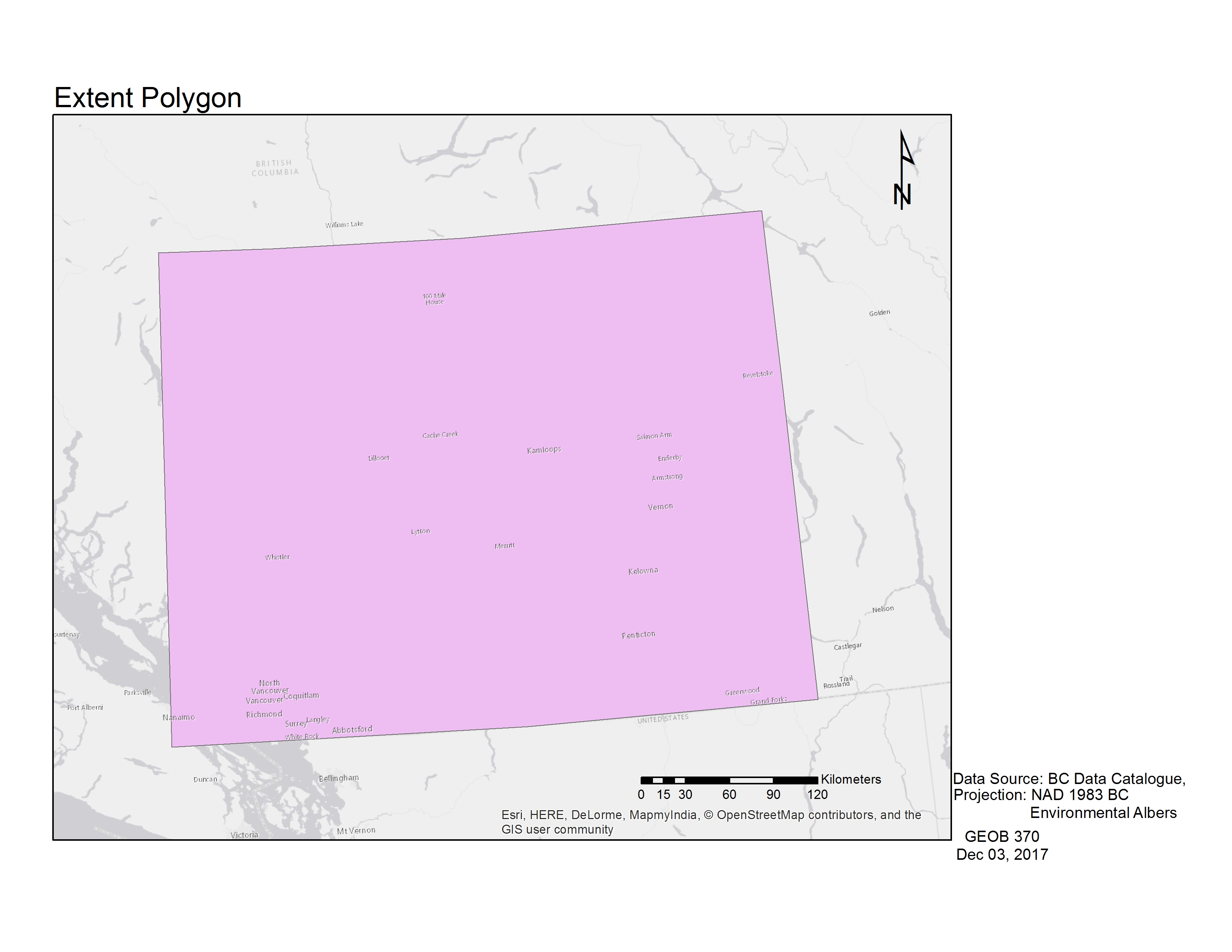
Fig 3. Map of the extent polygon utilized for data acquisition and clipping.
To create a layer encompassing human activity and development in BC, we went into the Other Land Cover layer and used the ‘Select by Attributes’ function to extract the developed land, perennial, and annual agriculture land use classes. This layer was used alongside the ‘Other Land Use’ layers acquired from DataBC in our MCE (Fig 4; Fig 5).
We then projected all our layers onto the NAD 1983 BC Environmental Albers coordinate system using the ‘Project’ tool, and at the same time we set the processing environment to match the cell size of the DEM we were using, in order to prevent any issues when converting our polygons to raster.
Until now almost our layers were in polygon or polyline form, so we then converted our polygon layers to raster, which was necessary in order to utilize them within a Multi-Criteria Analysis.
Once we projected our polygon layers, we then converted them to raster using the ‘Feature Class to Raster’ tool. Afterwards, we used the ‘Raster Reclassify’ tool to alter the values in the rasters so that they would represent the presence or absence of a feature on the map. We used the tool to set the cells where an objectID was present to a value of 1 and those which did not have an objectID for that layer to a value of 0. The resulting layer would have cells with only values of 1s and 0s for the entire extent of the map (Fig 4)
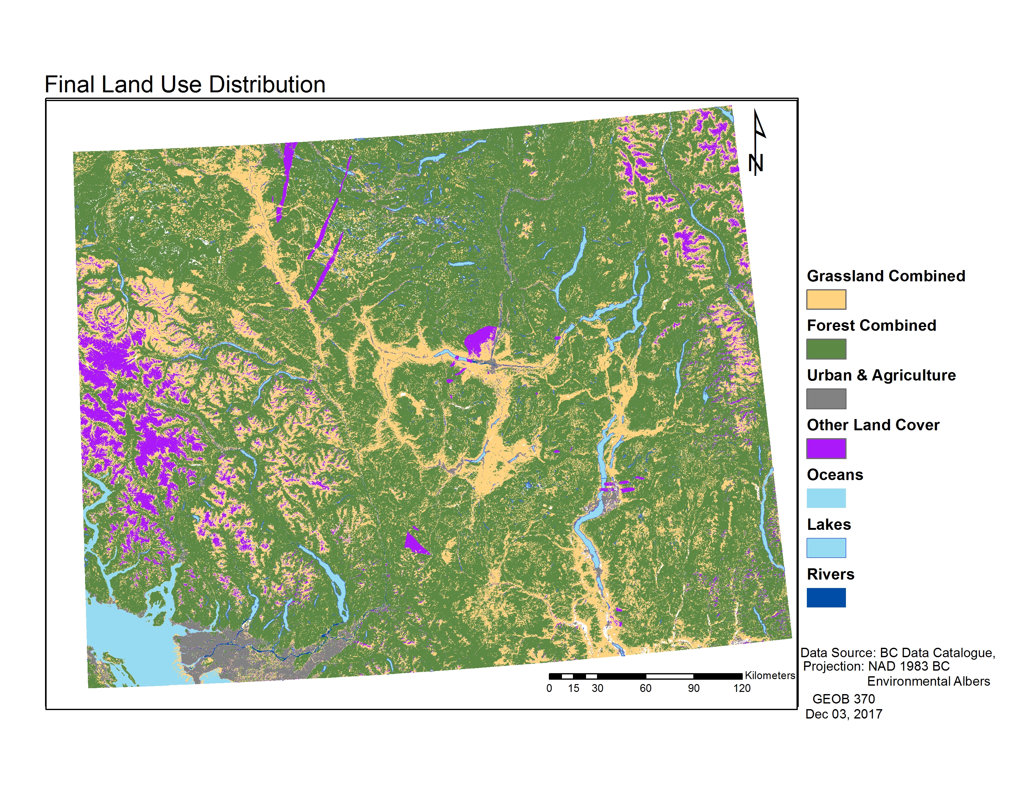
Fig 4. Map of final land-use categories of our B.C. extent, converted to raster format.
![]()
Fig 5. Map of major roadways, transmission lines, and water bodies
We utilized the ‘Slope Calculator’ tool to give us the slope from the DEM, and then used the ‘Map Algebra’ tool to score these slopes with values ranging between 1 and 0; with 1 representing the shallowest slope, and 0 representing the steepest slopes.
AHP Weighting
To complete our multi-criteria analysis, we used 123AHP to help determine the weightings to be given to different land features in our study area (Fig 6). We based our decisions on how passable a certain feature is for bears to travel through or live in. Our ranking places lakes and urban/agricultural land as being most unfavorable for bears, with grasslands and forests being the most favourable.
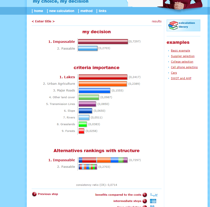
Fig 6. 123AHP results for our weighting decisions.
Grizzly Subpopulations
To mark the areas of currently occupied habitat, potential wildlife corridors, and possible reintroduction sites we chose zones/corridors in our maps which scored well in our MCE. To highlight these high-scoring areas we used the editor feature to draw polygons that matched the shape of these areas (Fig 7).
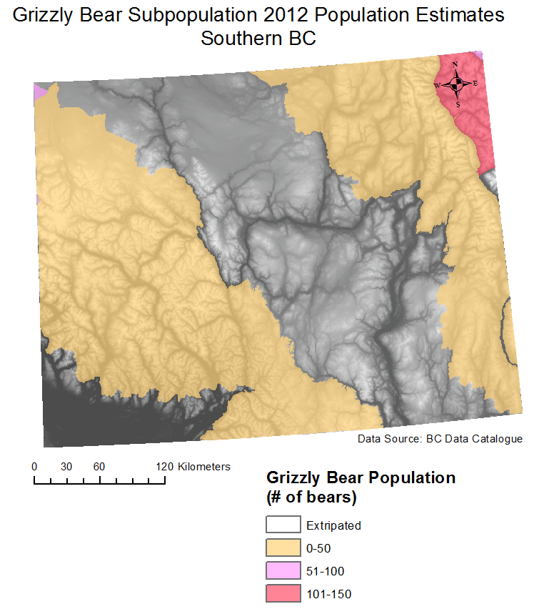
Fig 7. Map of combined subpopulation areas and abundance estimates, overlaid on the DEM.