Data Acquisition
After identifying a research question and area of interest, my first step was to identify what data I needed to complete my analysis. I examined provincial mountain resort guidelines, similar examples of GIS analyses, and ski resort master plans to determine what types of data I would need. Page 9 of the 2006 BC Mountain Resort guidelines states that ski resort site inventory and analysis should involve the following steps: ‘Delineate and describe existing [land] use”, “Delineate legal boundaries”, “Delineate and describe adjacent land use”, “Research existing tenures”, “Slope analysis by skier skill classification breakdown”, “Elevation Analysis”, “Review accessibility”, “Aspect Analysis”, “Skiing Potential” and “Climate/snowpack analysis” From these guidelines I identified six types of data that would be most important for determining physical ski slope potential and accessibility:
- Elevation
- Slope
- Aspect
- Land Use
- Snowfall
- Distance from Roads
I primarily acquired data from provincial and national Canadian open data catalogues. For example, I acquired a 20-meter digital elevation model (DEM) and 2010 land use data from the Canadian government open data portal, and a digital road atlas and environmental region data from DataBC which is the province’s official data catalogue. There was no available data for a snowfall surface across the province, so I acquired snow station data from the BC River Forecast Center website and snow station locations as a shapefile from the UBC ABACUS network.
I decided on using the NAD83 BC Albers projection for my data, since this is a standard for BC centered mapping that is used for mapping the entire province or for smaller areas within BC. All data was projected to BC Albers if necessary. Continuous raster data (such as the DEM) was resampled bilinearly, whereas discrete raster data (such as land use) was resampled using nearest neighbor. All data was imported into a file geodatabase.
Data Derivation
Some of the identified data needed to be derived rather than directly acquired. I derived the Aspect data from the DEM using the ‘Aspect’ tool in ArcGIS, and the Slope data from the DEM using the ‘Slope’ tool in ArcGIS. In order to create the snow surface data, I averaged the 5 year hourly measurements from the 2011-2016 raw snow water equivalent data for each station and created a new table with the snow station number, name, and average snow water equivalent measurement. I then joined this table to the snow station location shapefile, removed stations for which there was no snow data (such as the manual, non-automated stations), and imported this file into my geodatabase. This produced a point feature class showing the locations of 62 of the automated snow stations that each had average snow water equivalent data. From this I used the trend tool with linear regression and a polynomial order of 2 to roughly interpolate snow water equivalent across the entire province, and then clipped the resulting 30 meter raster to the study area. I used this rather than a more intensive interpolation method because the relatively low number of stations throughout the province could only be used to indicate a general pattern rather than create a detailed surface.
Capability Analysis
The first step in my analysis was to assess capability, by determining how much of the region of interest might be physically able to function as a ski slope in a resort capacity. I used three different types of data to perform this analysis: elevation, slope, and land use. The output was a binary classification of the entire lower mainland environmental region.
Elevation was considered for the capability analysis because below a certain elevation, there is simply no potential for sustained snow throughout the winter (i.e. enough for locating a ski resort). In order to determine the cut-off elevation for ski slope capability, I examined all of the ski existing resorts that were within my study area to see what their elevations were. The lowest base area (minimum lift-accessed skiable elevation) of all of these resorts was at Whistler Creekside, which has an elevation of 653 meters. I then reclassified the DEM, which had a range of elevation from -7 to 3462 meters, so that elevations from -7 to 653 had a value of 0 and elevations from 653 to 3462 had a value of 1.
Slope was considered for the capability analysis because downhill skiing/snowboarding is not possible on nearly vertical slopes or on very flat slopes. To determine what slopes could support skiing, I researched the master plans for existing ski resorts. The following table of ski slope classifications was found on page 84 of the Silverstar Resort Master Plan (2017):
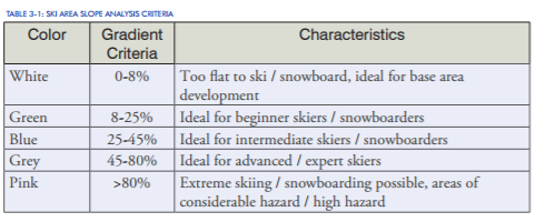
Using this information, I then reclassified the previously derived slope layer by classifying gradients of 0-8% as 0, 8-80% as 1, and 80-90% as 0. The gradients of each cell in the study area ranged from 0 to 83.997%.
Land use was considered for the capability analysis because areas that are already used for agriculture and settlement or covered in water or wetlands can not be feasibly converted into skiable slopes. I acquired a land cover raster data set with a 30 meter resolution through the government of Canada’s data portal. The land use data was produced in 2010, with the following classes as documented in page 7 of the ISO 19131 Land Use Data Product Specifications:
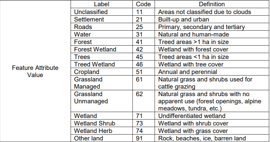
I considered the following classes unsuitable for ski slope development: settlement, roads, water, forest wetland, treed wetland, cropland, grassland managed, wetland, wetland shrub, wetland herb. I reclassified the data so that all of these classes were given a value of 0. The other classes which were unclassified, forest, trees, grassland unmanaged, and other land were all given a value of 1 to indicate capability.
After reclassifying each of these three datasets, I then used the raster calculator tool in ArcGIS to multiply each layer by the other. Given that each raster cell had a 1 or 0 value, the only cells with 1 value in the output raster were those that capable elevation, slope, and land use category.
The capable area that remained contained 20,825,407 cells, out of 48,382,263 total. This means that 43.04% of the total study area could potentially support ski slope development. Since each cell in the output capability raster was 30 x 30 meters, the total area of the capable region is 18,742,866,300 square meters, or 18,742.87 square kilometers.
Suitability Analysis
After performing a capability analysis to determine which areas could support skiing, I then moved on to a suitability analysis to assess which areas were better than others. I performed the suitability analysis using a Multi Criteria Evaluation (MCE) process. This involves combining normalized, weighted attributes in order to give cells a final ‘score’ that indicates how suitable they are. I referred to the MCE process for GIS laid out by Estoque (2011) when planning the various steps of this analysis. I focused on five criteria that pertain to slope skiing and access potential: elevation, slope, aspect, snowfall, and major road proximity.
For elevation, I simply considered higher elevation preferable to lower elevations for ski slope suitability, due to higher elevations tending to receive more snow and have lower temperatures. I therefore normalized the 20 meter DEM using the Fuzzy Membership tool in ArcGIS. This tool transforms the input raster to a range from 0-1, where a value closer to 1 indicates greater membership in a set or in this case greater suitability. I used the ‘Linear’ membership type, which linearly transforms the input raster (the lowest value becomes 0 and the highest value becomes 1).
For slope, I considered that intermediate level runs were the most conducive for skiing activities, with more extremely steep and flat slopes being less conducive. Referring to the previous chart listing ski area slope analysis criteria, I found that the intermediate category had grades of 25% to 45%, and therefore the most intermediate slope would have a grade of 35%. I again used the Fuzzy Membership tool to give the raster an 0-1 range. I used the Gaussian membership type (where values decrease with distance from the midpoint using a normal curve) with a midpoint of 35 and a spread of 0.001.
For aspect, I determined from my sources that northerly aspects are preferable for ski slopes because less sun exposure increases the amount of snow found on a slope. Aspect was more difficult to normalize because it ranges from 0 to 360 degrees, and ‘northerly’ slopes are at both extremes of this range. I therefore used the Fuzzy Membership tool with a Gaussian membership twice: once with a midpoint of 360, and once with a midpoint of 0. A spread of 0.001 was used for both. I then used the raster calculator to add the ‘high’ aspect raster to the ‘low’ aspect raster, so that very low and very high aspect values both were given high membership values.
For road distance, I first used ‘select by attributes’ to select roads that had a road class of highway, freeway, or arterial. I considered that proximity to a major road is important for a ski slope to be accessed by the general public. I then extracted these features into a new layer in ArcMAP, and the used the Euclidean Distance tool to create a 30 meter raster surface that indicated distance from the nearest major road. I used the Fuzzy Membership tool with an inverse ‘Linear’ membership type to normalize the distances from 0-1, where shorter euclidean distance values were given higher suitability values.
For snowfall, I used the derived snow water equivalent trend raster to indicate where higher average snow depths were likely to be found. Higher values indicated better suitability for ski slopes because they meant that snow lasted longer throughout the year and/or tended to be deeper. I used the Fuzzy membership tool with a ‘Linear’ membership type to normalize the interpolated average snow water equivalents from 0-1.
After creating these 5 normalized layers, I combined them using the Weighted Sum tool. This tool is used to overlay several rasters by multiplying them by their given weight and then summing them together. Since I did not determine or have evidence to indicate that any of the criteria were more important than any other, I gave each layer an equivalent weight of 0.2 so that the output raster would also values ranging from 0-1. After generating the output raster, I then used the raster calculator to multiply the weighted sum raster by the capability raster in which capable areas had a value of 1 and non-capable areas had a value of 0. The resulting raster showed ski slope suitability up to a maximum hypothetical value of 1, with all of the non-capable now having a value of 0. To display the final suitability output, I hid all of the 0 values by displaying as ‘no color’ to show only the capable area.
Identifying Best Sites
After producing the suitability map for the region, I identified specific regions with clustered high suitability values to determine the best potential sites for a new ski resort. To perform this function I used the Locate Regions tool in ArcMap. This tool uses a region-growing algorithm starting with certain seed cells to generate regions that meet a certain shape and evaluation method. I used the highest average evaluation method to create a 30 region output layer using the following inputs:
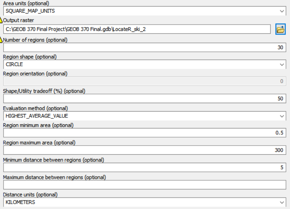
This produced an output raster with 400 meter aerial unit showing 30 ‘best’ regions for suitability indicated, with a generally circular shape for each region. I chose to examine the 3 best regions, which had the criteria of being between 0.5 and 300 square kilometers and at least 5 kilometers apart from any other identified region. I named these three regions based on nearby towns or features.