Data Preparation
In any GIS process, the first step is finding the appropriate data and checking their projections and coordinate systems. Please see our Data page for data sources.
- First we searched popular tourist locations, with the idea that people would want to rent bikes to go to these spots. We projected the lat/long from this data to create a data point tourism layer through Arc Catalogue.
- Secondly we downloaded the CHASS census data for population density as one of our criteria for the MCE. We had a challenge in joining the census table to our Dissemination Areas layer and learned that you have to import an excel file (.xlxs) not a CVS file if you want to keep the text formatting for the DAUID.
- Next we merged the layers of skytrain stations and public transportation stops.
- The rest of the layers were ready to input such as roads, parks and lakes with minor changes in symbology, and the city mask.
- Finally, we clipped all the layers to our city mask extent.
Analysis – Part I
1. Population Density
After downloading the 2011 census as a csv file from CHASS, we added the table in and joined it with the Dissemination Areas (DA) layer of Vancouver using the field DAUID or GEOUID in CHASS, and changed the symbology to represent it appropriately. At this point, the layer is in DA polygons, and we need to rasterize it give it a fuzzy membership, so we converted it from polygons to a raster.
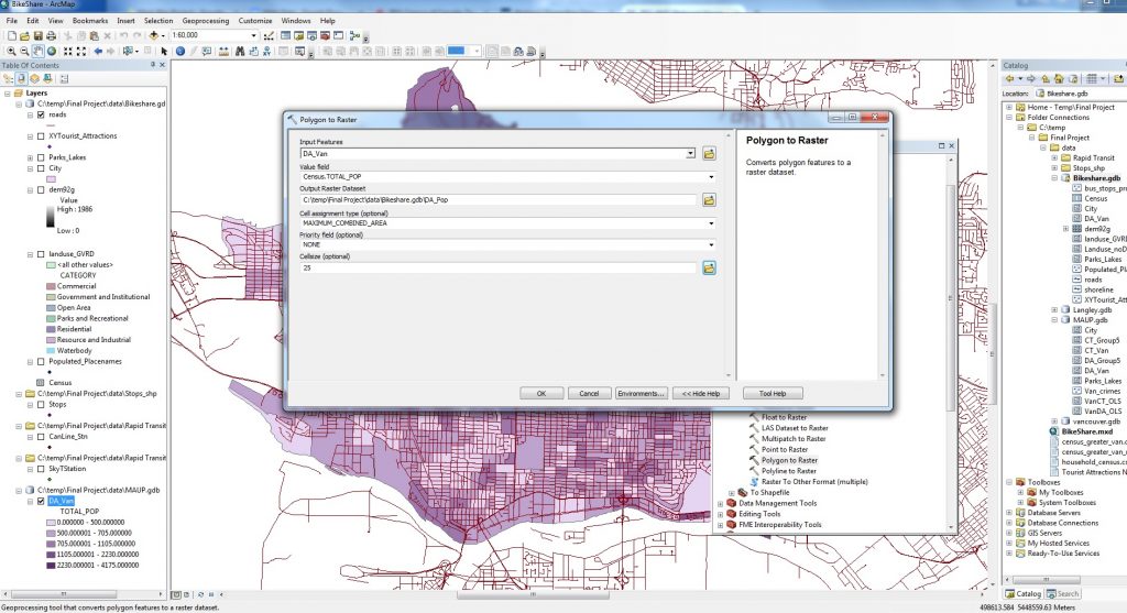
Figure 1. Depicting to Raster Conversion of Population Density
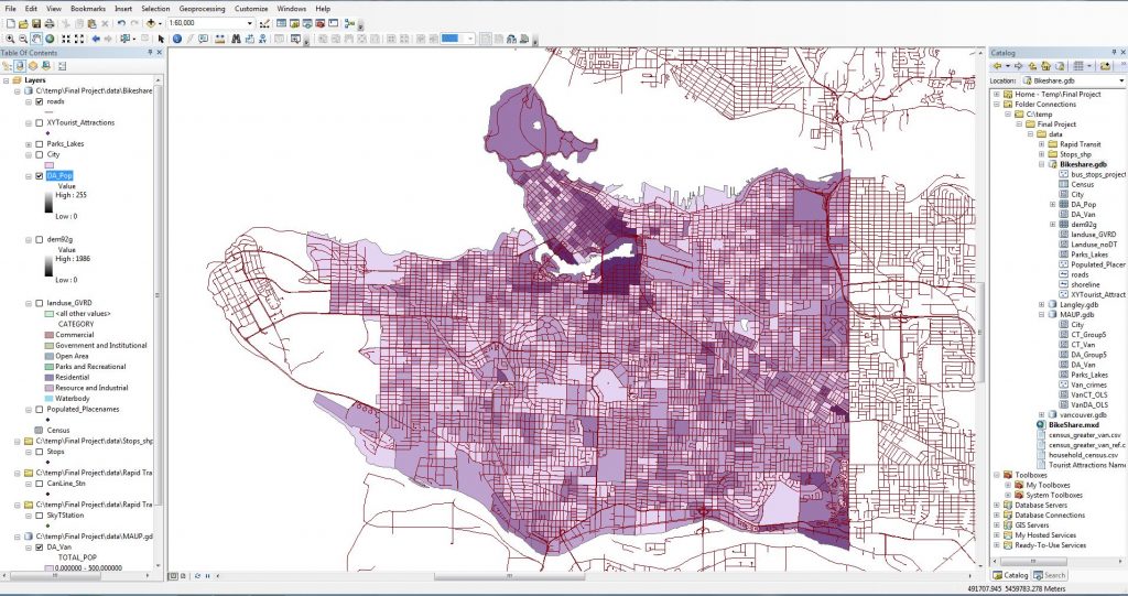
Figure 2. Population Density as Raster
Next we used the fuzzy membership tool to normalize the factor to be used in the weighted sum in our MCE. Unlike our second lab where we used the Gaussian selection, we used Large to imply that a high population density would have high membership.
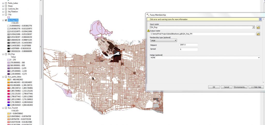
Figure 3. Fuzzy Membership for the population density raster
2. Public Transportation
With three layers of public transportation, we joined the bus stops, to the Canada Line Stations, and to the Millenium and Expo Line Stations, and rasterized it by using the Euclidean Distances tool. However, because of the density of those points, all the values came out looking the same, hence the entirely black layer.
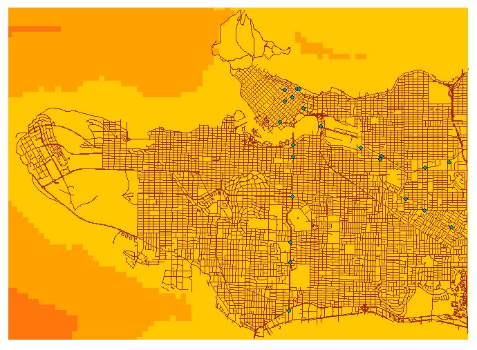
Figure 4. Euclidean distance raster of all transit including bus stops.
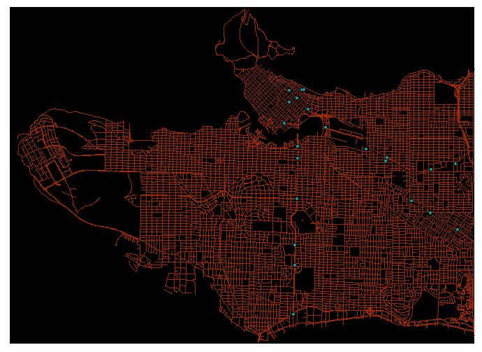
Figure 5. Fuzzy Membership of all transit stops with roads and train stations overlaid.
So in order to fix this, we took out the bus stops from the layer and decided to focus solely on the combined train stations. When we narrowed down to train stations, the information from the layer became a lot more valuable a criteria for our MCE.
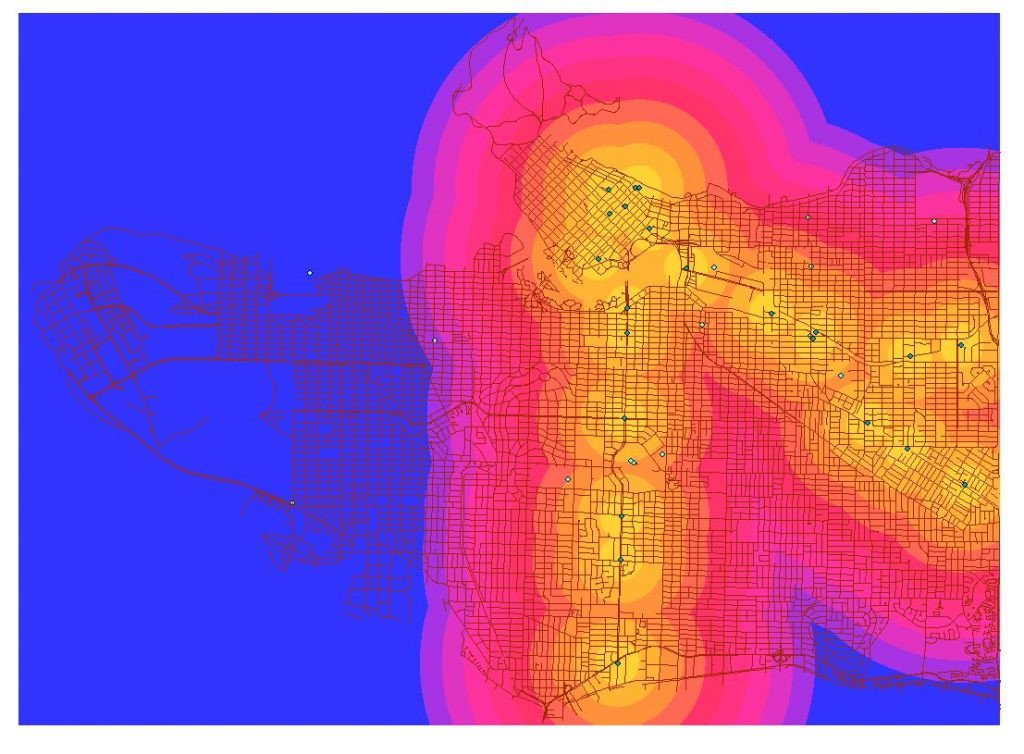
Figure 6. Euclidean distance of rapid transit (all train stations within Vancouver).
3. Tourist Attractions
At first, this was meant to be a mixed layer of both tourist attractions and parks; however with all the parks that dot Vancouver, the layer looked as useful as the full transit fuzzy membership (all one class of black). To remedy this, we divided this criteria into two. This layer then, focused solely on the tourist attractions that we identified and projected.
In line of the same idea, we needed to take our point layer and convert it into a raster to be normalized in the fuzzy membership tool.
Our first attempt introduced a problem with our extent. Without the full coverage of the raster layer, we would not be able to calculate outside of this raster when we got to the weighted sum. This was fixed in Geoprocessing Environments, under the processing extent tab, but we also selected the extent to match our city mask in the tool’s environment option just to be doubly sure.
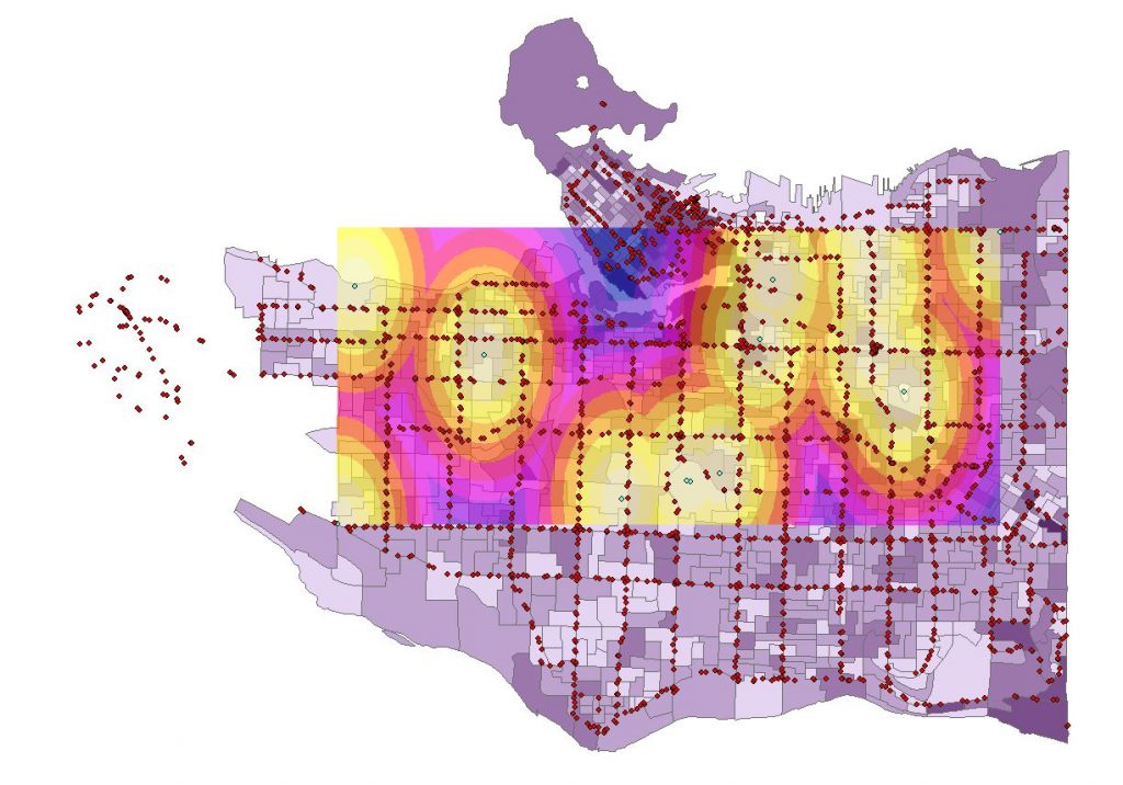
Figure 7. Euclidean Distance from tourist locations. We had a problem with the raster extent of the layer.
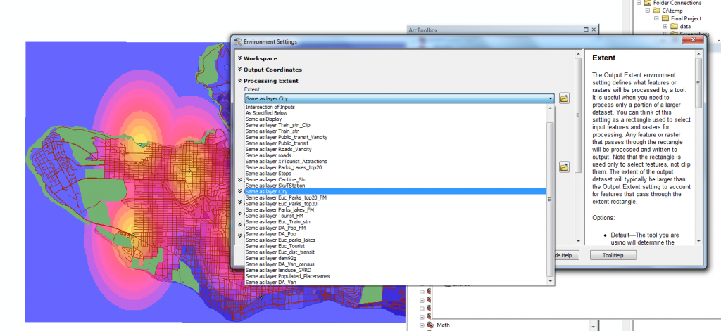
Figure 8. Fixing the processing extent.
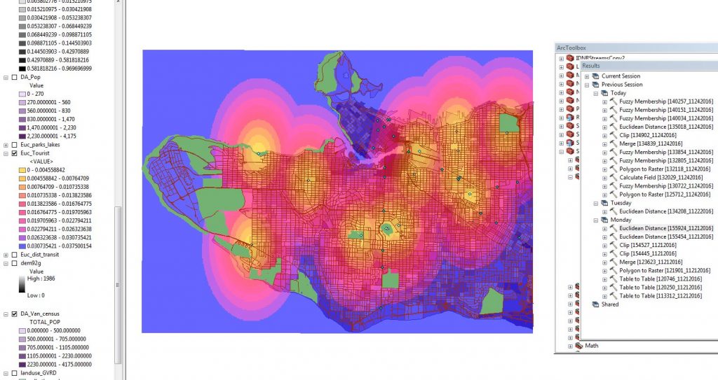
Figure 9. Euclidean distance for tourist locations with a fixed processing extent.
4. The 20 Largest Parks in Vancouver
To avoid creating a useless criteria layer, we queried in the parks and lakes layer for parks larger than 200,000 meters squared and selected the 20 largest parks, as you can see in Figure 10. We then proceeded to rasterize and normalize it.
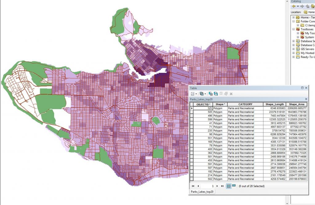
Figure 10. The 20 largest parks in Vancouver.
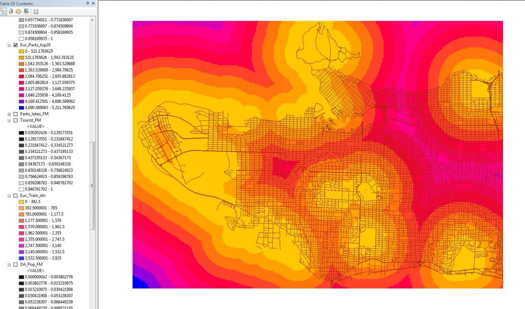
Figure 11. Euclidean distances around the largest parks.
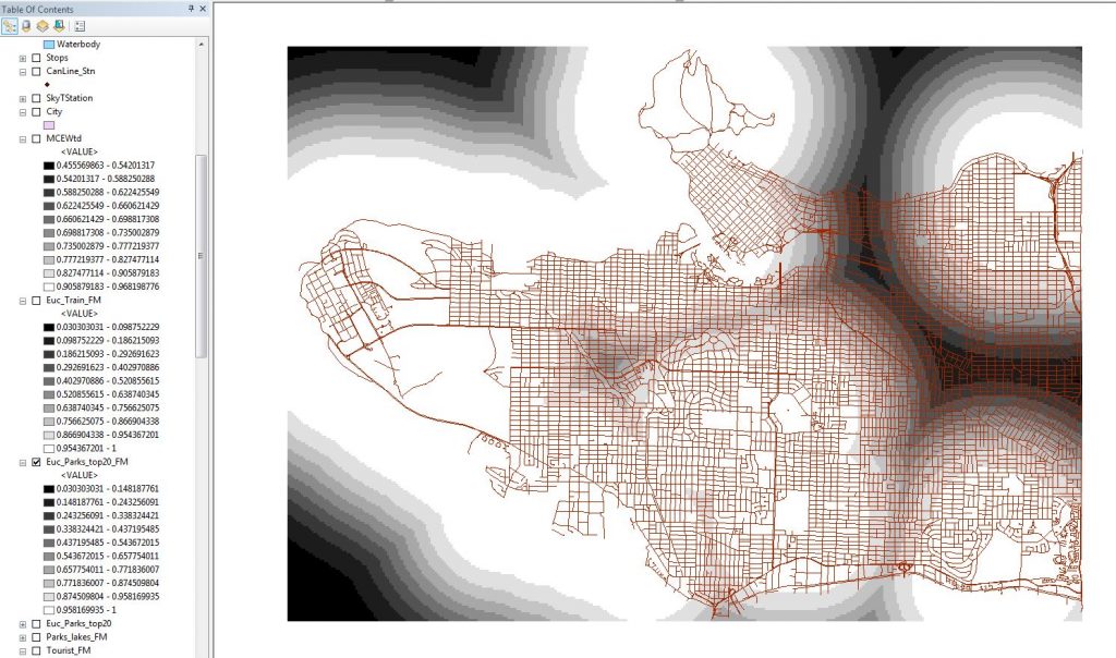
Figure 12. Fuzzy membership of largest parks. White are the values of highest membership (close to the parks), and black is far away from the parks (low membership).
Analysis – Part II: MCE
Deciding the Weights
To decide what weights to use, we returned to the AHP we used in lab 2, and inputed the weights as below.
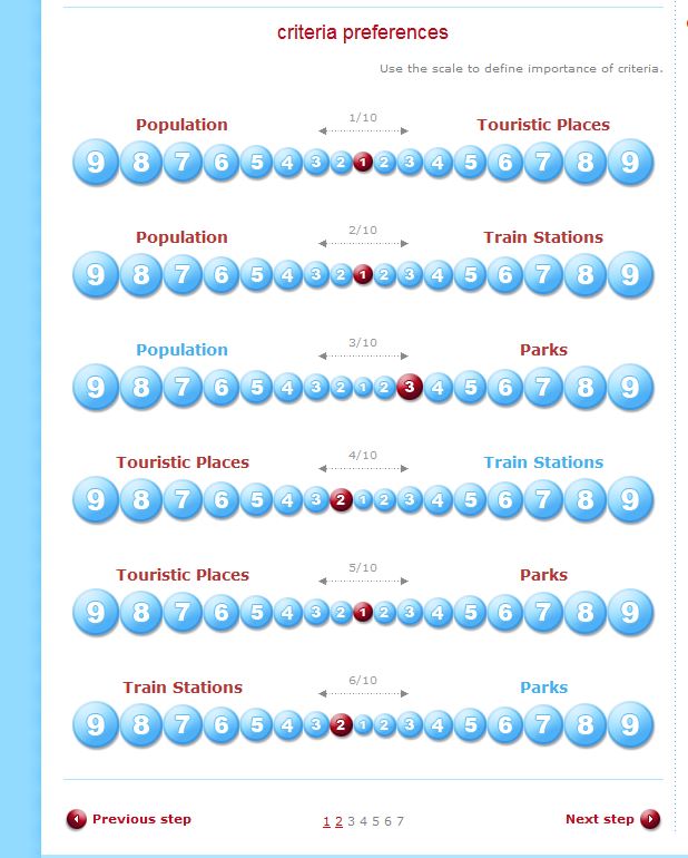
Figure 13. Selected weights

Figure 14. AHP results.
Weighted Sum
Using our 4 criteria: high population density, proximity to train stations, touristic sites, and large parks, we used the weights we got from the AHP, and created the weighted sum layer.
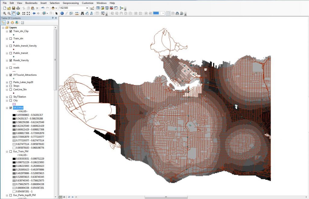
Figure 15. Weighted Sum
Post Analysis: Creating Bike Station Locations
Raster-to Point for the MCE
- After converting the MCE layer to a new raster cell size of 250m x 250m for easier analysis of the points, we converted the raster to a point through Conversion Tools-> From Raster -> To Point
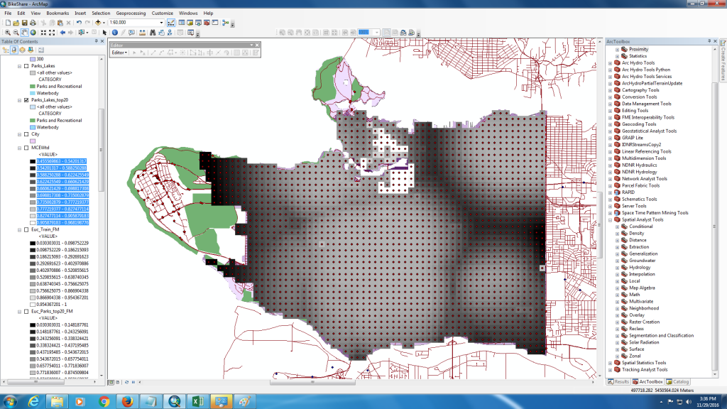
Figure 16. Raster to Point Conversion
- A Tree Hugger article on the success of bike shares noted that successful bike shares have stations a convenient walking distance apart, about 300 metres (Alter, 2013) for high density areas. Additionally in a study by Castillo-Manzano et al. (2016), the researchers confirmed that in dense city areas, an average distance of 300 metres was found between stations. Based on our scale, we decided that the areas (in white) that are most suited for a bike share location based on the MCE should be 250 metres apart, while locations that are less ideal, but may still require a bike share station should be about 6000m based on the distance to bike in 20 minutes being about 6000m, leading us to believe that would be the distance required for less-suspected to be used areas. The range was based off of the Frequency Distribution.
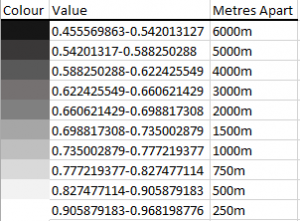
Figure 17. Distance between stations based on the MCE
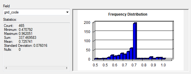
Figure 18. Frequency Distribution of values based on MCE
Station Selection
- Unfortunately there are no tools available that easily spread out points based on our analysis above, therefore as suggested by Dr. Klinkenburg we hand edited the points based on the previously discussed distances. The colours were changed for easier viewing where the darkest blue colours signify the most desirable locations and the red locations are the least desirable. Then the points were joined to the roads using Proximity -> Near.
- A Tree Hugger article on the success of bike shares noted that successful bike shares have stations a convenient walking distance apart, about 300 metres (Alter, 2013) for high density areas. Additionally in a study by Castillo-Manzano et al. (2016), the researchers confirmed that in dense city areas, an average distance of 300 metres was found between stations. Based on our scale, we decided that the areas (in white) that are most suited for a bike share location based on the MCE should be 250 metres apart, while locations that are less ideal, but may still require a bike share station should be about 6000m based on the distance to bike in 20 minutes being about 6000m, leading us to believe that would be the distance required for less-suspected to be used areas. The range was based off of the Frequency Distribution.
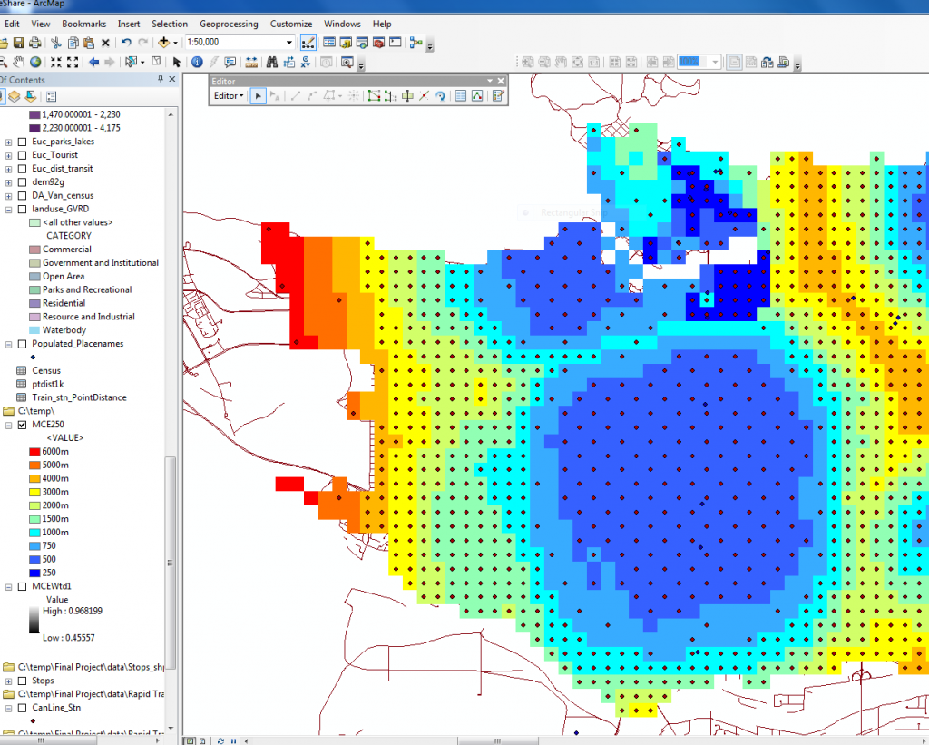
Figure 19. Points in the process of deletion. The colours were changed for easier viewing.
See our finished map in the Results Page.
