The DEM tiles were mosaicked into a single raster.
Following this flow chart until Flow Accumulation, Flow Direction was first calculated.
Sinks were identified and any 7m or less in depth were filled, following the methodology in this example to create a depressionless DEM.
Flow Direction was recalculated using the depressionless DEM.
The polygon layer for Burns Bog was converted to a raster using a calculated value field that assigned all cells within this layer a value of 0.
The land uses were reclassified using a ranked contamination potential scale of 0-4, with agricultural areas being a 4, and land uses such as wetlands being given a 0.
Raster calculator was used to overwrite the cells in the land use layer with those cells that overlapped with the bog raster layer.
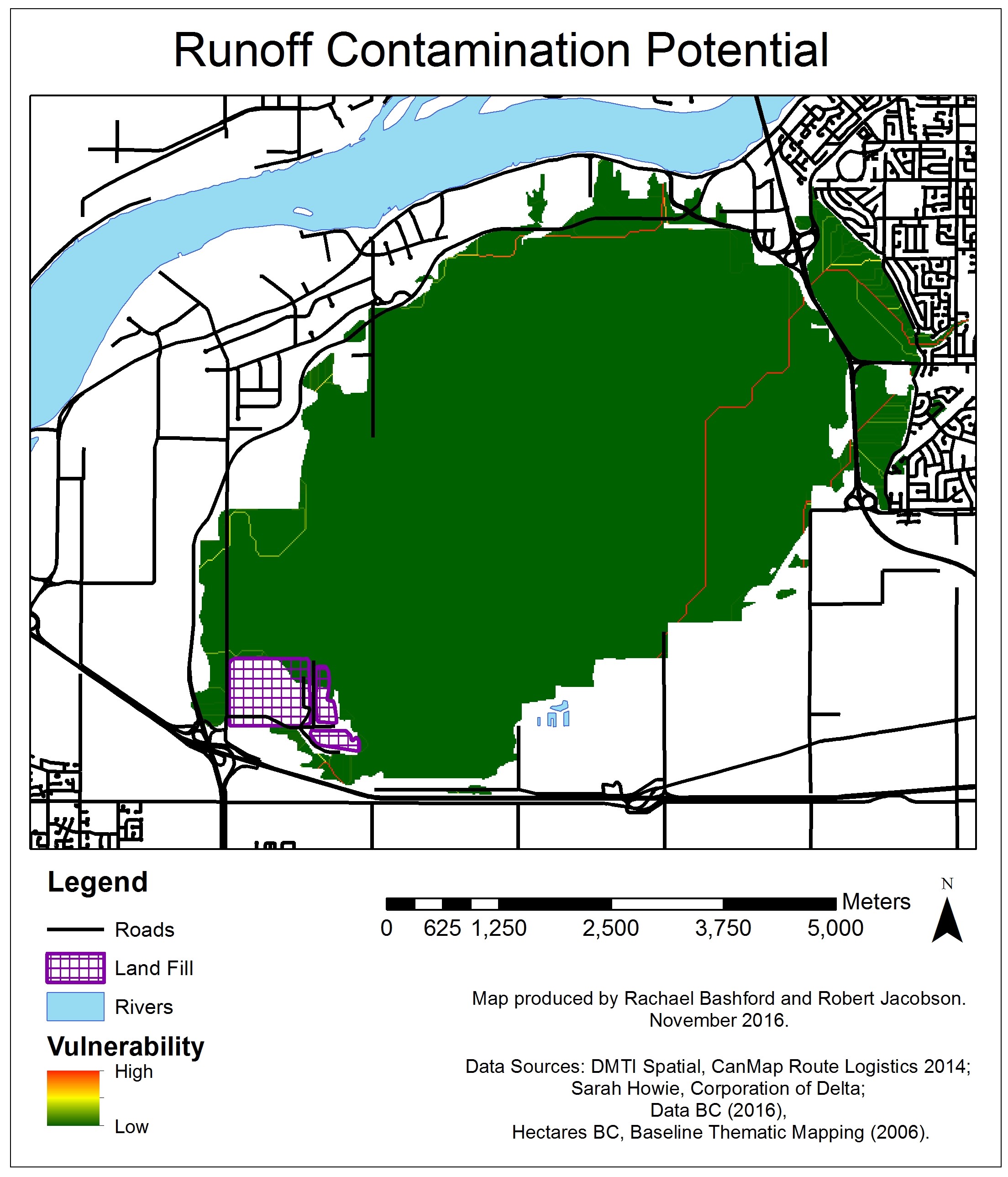
Flow accumulation was calculated using the land use raster as the weighted input layer (Figure 5).
To prepare the layer for the MCE, the layer was standardized using fuzzy membership with large values being closer to 1. The hedge was set to somewhat to account for potential error introduced by the relative contamination potential scale.