Author: byron hon
The purpose of Fitterer et al‘s paper, “Predictive crime mapping”, was to spatially predict commercial and residential break and entries (B&Es) in Vancouver, Canada. This paper aims to present a pilot project to have an automated model implemented within a mobile GIS that provides continually updated predictive maps to assist patrol units in self-deployment decisions. The data used for the study consisted of commercial and residential B&E data (provided by the Vancouver Police Department), population data from the 2011 Census and LandScan (ambient population), road network and land use data, graffiti data as a proxy for ‘lawlessness’, and data on average property values and house types were also used.
Fitterer et al’s methods suggested that an exploratory analysis was done in examining the space-time patterns of Break and Enters between 2001-2012, and a density map of BNEs was used to examine spatial patterns and hot spots. Furthermore, Ratcliffe’s near-repeat calculator was used to measure the spatial and temporal distance between each residential and commercial crime event that occurred (Fitterer et al, 2014). Based on observations made in assessing B&Es within 500m, 850m and 1000m from the original event and from one to 30 days since the event, two predictive models were developed for B&E crimes. Model 1 (Residential and Commercial) was based on integrating crime data with additional data using a generalized linear logistic regression estimation, while Model 2 was based only on observed crime data. Model 2 also assessed variable importance using the Knox ratio statistic, and assessed variable correlations to ensure models were statistically robust (Fitterer et al, 2014). Model accuracy was also assessed by visually comparing between observed and predicted spatial patterns. For Model 1, eleven data sets were found to be statistically significant predictors for residential BNEs, and 14 for commercial B&Es. These included B&Es within 850m from the event within the last 24 hours, 48 hours and seventh day, proportion of historical crime by time and day, road density, property value and type, count of B&E crimes in each cell, ambient and census population, and graffiti rate (Fitterer et al, 2014).
The results of the exploratory analysis found patterns in the characteristics of BNEs, including a progressive decrease in annual trends in the frequency of B&Es for both residential and commercial property types. On an hourly basis, residential offences decreased between 1:00 – 6:00, when residents were most likely to be at home, and peaked at 8:00, 12:00, and 18:00. Commercial B&Es occurred most often during 3:00, 4:00, 5:00, 17:00, and 18:00, while offences decreased during daylight hours (6:00-16:00). Spatially, the authors found consistency in patterns between 2001 and 2012, with Downtown parts of Vancouver having the majority of residential B&Es, with sections of the Westend and area around the Downtown core (Strathcona, Kitsilano, Fairview, Mount Pleasant, Oakridge, and Marpole) suffering from high numbers of property crime. Moreover, spatial consistency was found in commercial B&Es, with clusters around the Downtown neighbourhoods and surrounding regions of Fairview and Mount Pleasant, and local hot spots in the southern Arbutus ridge and Marpole areas. Overall, the results indicated that within short spurts of time and nearby vicinity of a break and enter, there is a high possibility of another break and enter occurring as well.
The limitations of the model are indicated by Fitterer et al., which includes the relatively rare occurrence of B&Es, spatial autocorrelation, and the difficulty to predict crimes at fine spatial resolutions due to the importance of scale between 850 m to 500 m (Fitterer et al, 2014). The methods portion of the paper also lacked any thorough explanation, specifically about the minimization of model choice bias through the use of considerations like AICc and Bandwidth parameter, or any other kinds of model accuracy evaluation. Due to this, I decided to give this paper an 8/10.
Article: Predictive Crime Mapping by J. Fitterer, T.A. Nelson & F. Nathoo
http://www-tandfonline-com.ezproxy.library.ubc.ca/doi/full/10.1080/15614263.2014.972618?needAccess=true
The article I reviewed for this section is called “Analyzing spatial clustering and the spatiotemporal nature and trends of HIV/AIDS prevalence using GIS: the case of Malawi, 1994-2010” and the aim of the study was to:
- Examine spatiotemporal trends in HIV prevalence from 1994 – 2010
- For 2010, it identifies and maps the spatial variation or clustering of factors associated with HIV prevalence at the district level in Malawi
The methods used for this study required 4 main steps:
-
- Obtaining HIV prevalence data and temporal trends at national, regional and urban/rural scales
- Determining spatial dependence in HIV prevalence, spatial interpolation, and spatiotemporal trends
- First, the HIV prevalence rates for the pregnant women were plotted (from 1995 to 2010) to provide a spatiotemporal perspective of the HIV epidemics at its various levels (national, regional, urban and rural).
- Then, they used GIS tools to
- Empirically test for spatial dependency in HIV prevalence nationally
- Produce a continuous surface of HIV prevalence at 1 x 1 km spatial resolution for visualization and generation of prevalence estimates at district level for cluster/hotspot and regression analysis.
- HIV spatial autocorrelation was also assessed using global Moran’s I statistic
- Which is indicative in suggesting whether HIV clustering occurs in a hierarchical expansionary spread in different areas and districts.
- The Inverse Distance Weighted spatial interpolation method was used for the years 1994, 1996, 1999, 2001, 2003, 2005, 2007, and 2010.
- uses weights based only on distance between measured and unmeasured points
- IDP assigns more influence to measured values nearest an unmeasured location than to measured values located farther away
- Local spatiotemporal variation in HIV prevalence and cluster/’hotspot’ analysis
- Regression analysis and indicative drivers of HIV prevalence for 2010
For the results, the analysis revealed that there was a wide spatial variation of HIV prevalence at a regional, rural/urban, district and sub-district levels. However, prevalence was spatially plateauing out within and across ‘sub-epidemics’ while declining significantly after 1999. Prevalence showed statistically significant spatial dependence nationally following initial (1995-1999) localized, patchy low/high patterns as the epidemic spread rapidly. Locally, HIV “hotspots” clustered among eleven southern districts/cities while a “coldspot” captured configurations of six central region districts. Preliminary multiple regression of 2010 HIV prevalence produced a model with four significant explanatory factors (adjusted R2 = 0.688): mean distance to main roads, mean travel time to nearest transport, percentage that had taken an HIV test ever, and percentage attaining a senior primary education. Spatial clustering linked some factors to particular subsets of high HIV-prevalence districts.
I rate this article a 8/10 due to the limitations of the study which was also referenced within the article. The small sample size of 19 sentinel ANCs is not optimal as well as the use of OLS regression model was just sufficient enough and left out the spatial lag model findings.
The article I wrote about entails using ecosystem service values to assess the ecological values of corresponding land-use types, essentially to evaluate the ecological effects of regional land-use change within the study area of Yongsheng County in north west Yunnan Province between the years 1988 – 1999.
The main objective that was noted by the author were to: “(1) identify land-use change processes in China’s southwest agricultural landscape within the past 11 years through analysis of the dynamics of landscape metrics; and (2) consider relative changes from the global mean economic value of the ecosystem service in order to evaluate the ecological effects of LUCC.” (Peng et al, 2006, 317).
Land use/land cover change (LUCC) not only results in changes to the landscape structure of the Earth’s surface, but also influences material cycles and energy flow in the landscape, and biodiversity and important ecological processes in a region. This makes it worthwhile to study the relationship between the LUCC and the eco-environment to understand potential changes in the regional ecological environment. Assessing the ecological quality of regional land-use types according to the proportional relationship of the ecosystem service is necessary as well as then evaluating the ecological value change due to LUCC.
This methodological approach and the procedures used was appropriate for the research question as it analyzed land-use change with transition matrix identifying important processes, change in landscape diversity, and change in spatial configuration of landscape elements, change in patch shape. The ecological effects of land-use change were explored through integrated ecological effects of land use change in the whole country and spatial differentiation of ecological effects of land-use change. These factors all contribute to the arguments established by Peng et al that land-use change is largely existent due to human factors and affect ecological structures of the land. Due to the complexity and large scale of the paper, it is often very hard to articulate the grand scheme of the project into a concise and easy to understand manner. This paper should be commended for its easiness to read and follow through each procedure. For this reason, I would give this paper a 9/10. The only criticism would be its absence of translation of data into maps which would perfectly illustrate the results of the findings.
Article: Ecological effects associated with land-use change in China’s southwest agricultural landscape. International Journal of Sustainable Development & World Ecology
Within this Lab we used CrimeStat to evaluate the spread of break and entry crimes and auto thefts in Ottawa, Ontario. The data was obtained from the National Institute of Justice’s CrimeStat 4.02, and results were visualized using ESRI’s ArcMap as well as Microsoft Excel. Firstly, a statistical analysis was performed using CrimeStat to calculate the different kinds of indices related to distance through using the nearest neighbour clustering and Moran’s I correlograms. Moran’s I deals with the predictability of crime across various Dissemination Areas whereas Nearest Neighbour looks at spatial clustering between actual points. Despite small differences, both Moran’s I and Nearest Neighbour appears to show decreased correlation as positioned further from the chosen area.
In terms of identifying hotspots, Fuzzy Mode, Nearest Neighbour Hierarchical Spatial Clustering, and Kernel Density Estimates were used. Fuzzy mode produces frequency points by analyzing crime form its surroundings. One advantage of Fuzzy mode is that it can identify hotspots without creating exact areas/points by sampling nearby points. For Nearest Neighbour Hierarchical Spatial Clustering, this method is split between two other methods: Standard and Risk-adjusted Nearest Neighbour Hierarchical Spatial Clustering, which both creates ellipses representing clusters of crime. Kernel Density Estimates is split between two methods: Single surface and Double surface. Single Surface maps absolute crime volume whereas Double surface maps and normalizes crime rate. The Knox Index was then used to look at space-time clustering for car theft data. It examined whether the thefts were close or far in space and time. 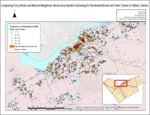
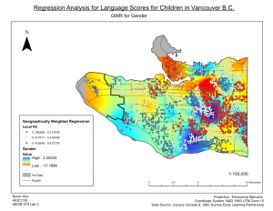
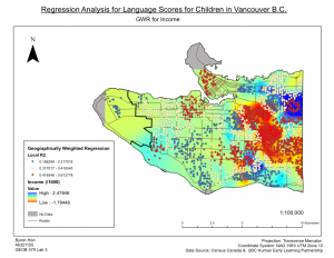
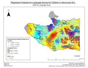
Within this lab, we assessed the factors that contribute to the social score outcomes of children, and how spatially consistent relationships between sociability scores and explanatory variables (family income, language skills, gender, and parental status) were across Vancouver using ArcMap. The data was obtained from Human Early Learning Partnership (HELP) at UBC, using Early Development Instrument (EDI) questionnaire. Moreover, census data (Enumeration Areas) was also used in the grouping analysis. An explanatory regression analysis was used to determine the set of variables that provides the best relations, with consideration of six explanatory variables(social score, percentage of neighbourhood families that are lone parents, percentage of neighbourhood immigrants that were recent immigrants, and percentage of neighbourhood that does not have French or English as their first language, % of the neighbourhood that belongs to a visible minority, and income). Three variables of the most significance were then determined: family income, language score, and gender. From this, an ordinary least squares analysis (OLS) was used to find a global model of sociability scores which was compared to the results produced by the Geographic Weighted Regression (GWR) tool. Grouping clusters were then determined using the Grouping Analysis tool to relate the results from OLS and GWR to other variables used to create the groups. I found that only two of the three variables are statistically significant from OLS, and the map of OLS residuals showed no significant spatial patterns. As for the GWR results, the surface map of social score showed good correlation with GWR R2 values, so it would seem that social scores and language scores have the strongest relation.
Lab 2: Exploring FRAGSTATS
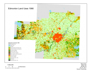
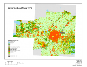
In this lab, land-use changes in Edmonton, Alberta between 1966-1976 was observed. We used FRAGSTATS to analyze the changes in land-use within Edmonton. The data used in this lab was obtained from the Canadian Land Use Monitoring Program (CLUMP), from Geogratis. There were multiple landscape metrics that were observed (Number of patches, Patch density, Shannon’s Diversity Index, Shannon’s Evenness Index, Landscape Division Index, and Total Edge) which were used to summarize overall trends of land-use change based on the whole study area. Followed by that, Class metrics (Class area, Percentage of landscape, Number of patches, Total edge, Total core area, and Largest patch index). The transition matrix showed exactly how each portion of land-use changed, and how the development of Edmonton was not only at the cost of cropland or improved pasture/forage crops, but other land uses such as mines, quarries, sand and gravel pits, and non-productive woodland. The comparison between the maps showed that there is an increase in urban built-up area, with urbanization appearing to radiate from the core from 1966 to 1976.
Within this lab, a yearly hot spot map of heart disease in the Southern United States was created with the data (ranging from 1999 – 2005) provided by CDC Wonder Data as well as Model Building in ArcGIS. First a model was created to process the data into individual feature classes, which was then followed by a second model to perform a hot spot analysis on each year’s feature class. Lastly, the yearly hot spot feature class maps was also animated. The main focus of this lab was to review how to properly create a map using adequate map formatting and elements.
March 1 – 3: GIS and Crime
GIS is an important tool for crime analysis as it allows law enforcement agencies to understand crime data from a geographical spatial perspective by visualizing the occurrence of crime and analyzing the spatial patterns of crime. Crime analysis is defined as the qualitative/quantitative study of crimes as well as law enforcement information with relation with socio-demographic and spatial factors to arrest criminals, prevent crimes, reduce disorder, and evaluate organizational procedures. The different kinds of crime analysis includes intelligence analysis, criminal investigative analysis, tactical crime analysis, and strategic crime analysis.
Crime is argued to be a geographical problem due to the fact that it depends on the activities of people, which is operated often at a routine basis. Routine activity theory predicts that residential homes are burglarized during the weekdays in the daytime and commercial properties during the weekend and nighttime hours, due to routine of temporal pattern of vacancy within a certain space. Sociodemographic and socioeconomic characteristics of people are not random, so routine activities are also not random. Criminal pattern theory states where and when the offence will occur. Rationale choice theory suggests that as offenders are influenced by the daily activities and routines of their daily lives, they tend to stay in areas that are familiar to them. These 3 theories are part of the field of environmental criminology.
There are 4 major applications of GIS in health geography: spatial epidemiology, environmental hazards, modelling health services, and identifying health inequalities. Spatial epidemiology is focused on the understanding of spatial patterns in disease. As populations are spread unevenly, populations tend to be more fluid and people live in communities, which means, geography can play a crucial role in the spatial distribution of disease. They also help us understand trends and mapping variations. There are 4 major applications of spatial epidemiology: disease mapping, cluster detection, spatial exposure assessment and assessment of risk of disease. Environmental hazards both map hazards and help prevent future problems through analyzing exposure and outcome surveillance. Modelling health services and identifying health inequalities are interrelated as they both deal with mapping and identifying socioeconomic and demographic data.

