Category: GEOB 479 Labs

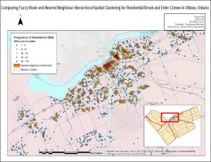
Within this Lab we used CrimeStat to evaluate the spread of break and entry crimes and auto thefts in Ottawa, Ontario. The data was obtained from the National Institute of Justice’s CrimeStat 4.02, and results were visualized using ESRI’s ArcMap as well as Microsoft Excel. Firstly, a statistical analysis was performed using CrimeStat to calculate the different kinds of indices related to distance through using the nearest neighbour clustering and Moran’s I correlograms. Moran’s I deals with the predictability of crime across various Dissemination Areas whereas Nearest Neighbour looks at spatial clustering between actual points. Despite small differences, both Moran’s I and Nearest Neighbour appears to show decreased correlation as positioned further from the chosen area.

In terms of identifying hotspots, Fuzzy Mode, Nearest Neighbour Hierarchical Spatial Clustering, and Kernel Density Estimates were used. Fuzzy mode produces frequency points by analyzing crime form its surroundings. One advantage of Fuzzy mode is that it can identify hotspots without creating exact areas/points by sampling nearby points. For Nearest Neighbour Hierarchical Spatial Clustering, this method is split between two other methods: Standard and Risk-adjusted Nearest Neighbour Hierarchical Spatial Clustering, which both creates ellipses representing clusters of crime. Kernel Density Estimates is split between two methods: Single surface and Double surface. Single Surface maps absolute crime volume whereas Double surface maps and normalizes crime rate. The Knox Index was then used to look at space-time clustering for car theft data. It examined whether the thefts were close or far in space and time. 

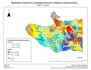
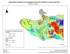
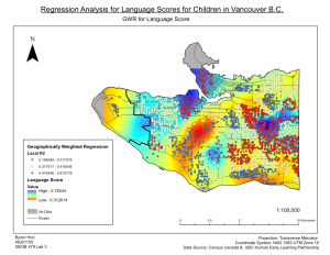
Within this lab, we assessed the factors that contribute to the social score outcomes of children, and how spatially consistent relationships between sociability scores and explanatory variables (family income, language skills, gender, and parental status) were across Vancouver using ArcMap. The data was obtained from Human Early Learning Partnership (HELP) at UBC, using Early Development Instrument (EDI) questionnaire. Moreover, census data (Enumeration Areas) was also used in the grouping analysis. An explanatory regression analysis was used to determine the set of variables that provides the best relations, with consideration of six explanatory variables(social score, percentage of neighbourhood families that are lone parents, percentage of neighbourhood immigrants that were recent immigrants, and percentage of neighbourhood that does not have French or English as their first language, % of the neighbourhood that belongs to a visible minority, and income). Three variables of the most significance were then determined: family income, language score, and gender. From this, an ordinary least squares analysis (OLS) was used to find a global model of sociability scores which was compared to the results produced by the Geographic Weighted Regression (GWR) tool. Grouping clusters were then determined using the Grouping Analysis tool to relate the results from OLS and GWR to other variables used to create the groups. I found that only two of the three variables are statistically significant from OLS, and the map of OLS residuals showed no significant spatial patterns. As for the GWR results, the surface map of social score showed good correlation with GWR R² values, so it would seem that social scores and language scores have the strongest relation.

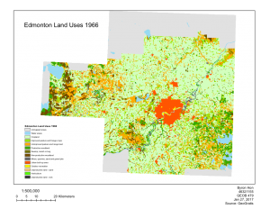
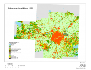
In this lab, land-use changes in Edmonton, Alberta between 1966-1976 was observed. We used FRAGSTATS to analyze the changes in land-use within Edmonton. The data used in this lab was obtained from the Canadian Land Use Monitoring Program (CLUMP), from Geogratis. There were multiple landscape metrics that were observed (Number of patches, Patch density, Shannon’s Diversity Index, Shannon’s Evenness Index, Landscape Division Index, and Total Edge) which were used to summarize overall trends of land-use change based on the whole study area. Followed by that, Class metrics (Class area, Percentage of landscape, Number of patches, Total edge, Total core area, and Largest patch index). The transition matrix showed exactly how each portion of land-use changed, and how the development of Edmonton was not only at the cost of cropland or improved pasture/forage crops, but other land uses such as mines, quarries, sand and gravel pits, and non-productive woodland. The comparison between the maps  showed that there is an increase in urban built-up area, with urbanization appearing to radiate from the core from 1966 to 1976.

Within this lab, a yearly hot spot map of heart disease in the Southern United States was created with the data (ranging from 1999 – 2005) provided by CDC Wonder Data as well as Model Building in ArcGIS. First a model was created to process the data into individual feature classes, which was then followed by a second model to perform a hot spot analysis on each year’s feature class. Lastly, the yearly hot spot feature class maps was also animated. The main focus of this lab was to review how to properly create a map using adequate map formatting and elements.