Click here for a direct link to the project website.
Abstract
The commute to the University of British Columbia can be thought of as a daily hassle. This project aims to provide insights towards the fastest and safest driving routes to and from UBC during peak traffic hours. In doing so, the map will help to inform the public of any areas to avoid in order to minimize their commute times and avoid accident prone areas.
The project used a kernel density analysis approach using ICBC accident data and ESRI’s ArcGIS software. Through analyzing crash severity and frequency, a ‘cost’ surface path was made. This enabled the production four respective paths leading from UBC to arbitrarily chosen points in Burnaby, Richmond, Surrey and Vancouver (which are different municipalities in the GVRD).
The intended audience of these results are faculty, staff and students of UBC. Further collaboration with ICBC, UBC and the municipalities would increase the accuracy of this project for its users. This project was conducted by Lucia Bawagan, Chelsey Cu, Tovi Sanhedrai and Lakshmi Soundarapandian as the final project of an Advanced GIS course (GEOB370) at UBC.
Introduction
In British Columbia, driving is regulated by the Insurance Corporation of British Columbia (ICBC), which was established in 1973 as a provincial Crown corporation. Since all vehicles are must be registered to legally be parked or driven on public streets in British Columbia, ICBC handles motorist insurance, vehicle licensing and registration, driver licensing, and produces annual traffic reports, statistics and crash maps.
The project, Safest Driving Routes from UBC to Areas Around the Greater Vancouver Regional District, was derived from our interest in finding the safest route from the University of British Columbia (UBC) to residential areas in the Greater Vancouver Regional District (GVRD). As driving is an important skill for most students and faculty members commuting to and from the campus, we take a special interest in road safety. The routes to each residential area are defined as the “least cost” paths that pass through areas classified under varying risk levels within an overall cost surface marked by car accidents that occurred in the previous year. These paths are created using ArcMap, and data from ICBC’s data catalogue.
The residential areas we have chosen are Vancouver, Burnaby, Richmond, and Surrey. These cities were chosen based on their variability in crash types and our assumptions that many people would commute from there to UBC. The least cost paths were created after a kernel density analysis to create a cost surface.
The goal of our project is to create a map of various least cost routes from UBC to residential areas in the GVRD. This map will hopefully bring awareness to young drivers, students and faculty about safe driving practices, frequency of car accidents and areas which have a high frequency of accidents.
Methedology
Initially, the task was to select four different cities within a Euclidean distance of 10 to 20 kilometers from the UBC campus. Settling on Vancouver, Burnaby, Richmond and Surrey, we used car crash data from ICBC along with lower mainland shapefiles, road networks and land use data to showcase the safest driving routes from these cities to UBC and vice versa. The method of analysis involved, first, data clean up prior to creating a cost surface, then selecting points in each city as a destination, before doing a kernel density analysis and creating a cost distance surface which is used to form the shortest, safest path from each city to UBC.
I. Data Clean Up:
The first step was to ensure that all the layers had the same spatial referencing. So, the projections were all changed to BC Albers and the datum to NAD 1983 UTM Zone 10. The layers were then added to the car crash data shapefiles creating the output layer. This was made into the main geodatabase. Then, the excel car crash data was imported into ArcMap and converted into a points layer in the geodatabase, using the command make xy event layer. Since this spatial referencing did not match, so the projection needed to be defined. We inputted the spatial referencing as WGS 1984 because the longitude and the latitude was measured in decimal degrees and we needed to convert it to meters in ArcMap for the car crash data shapefiles. At this point, other municipalities, that we did not intend to look at, also had data. So, those data points needed to be deleted while in the layer editing mode. The same was done for the roads that were outside of the Lower Mainland area prior to intersecting the layer to the main project layer.
II. Creating a Cost Surface:
Now, with the data organized, spatial analysis can begin. The cost factors were then defined, by assigning frictional values depending on frequency of car accidents in a location.
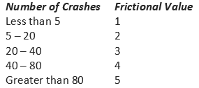
Table 1. Frequency of car crashes
Another set of frictional values were also added in for the severity of the car crashes.

Table 2. Type of car crashes
Also, the roads layer was converted into to a raster file and cost values were assigned based on if the pixel was part of a road (value of 1) or not a road (value of 0). During the processing, it was important to ensure that the calculations are restricted to roads (and do not incorporate waterways).
III. Selecting Source and Destination Features for the Route:
Since we did not have data on which specific neighbourhoods most people commuted from, an arbitrary point in each city was selected as a destination feature to avoid biases. This was done by doing a definition query, choosing points in layer editing mode, and deleting all other points that were not used. Once this was done, all the points in the different municipalities were merged into one layer.
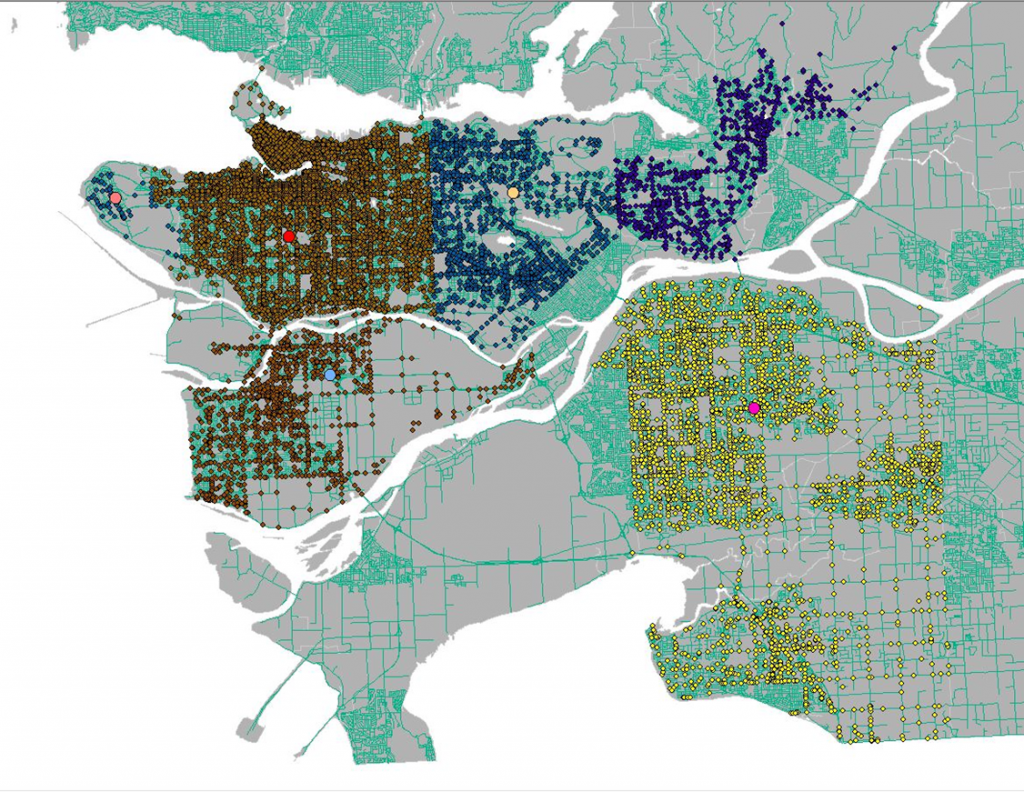
Figure 1. Accident points in municipalities and selected start points for safest routes (larger dots)
IV. Creating Cost Attribute:
The next step was to create a cost attribute by creating a new column in the attribute table that considers both the weight assigned to the number of crashes and the crash type. This was represented by seven classes in a gradient.
After this, a kernel density analysis was performed.
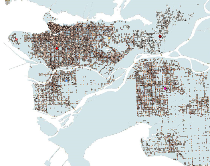
Figure 2. Combined attributes in preparation for the kernel density analysis
V. Creating Cost Distance Surface:
Next, we needed to create a cost distance analysis based on the new combined attribute that was made in the previous step. We created, not only a cost distance raster layer, but also the backlink raster layer as well.
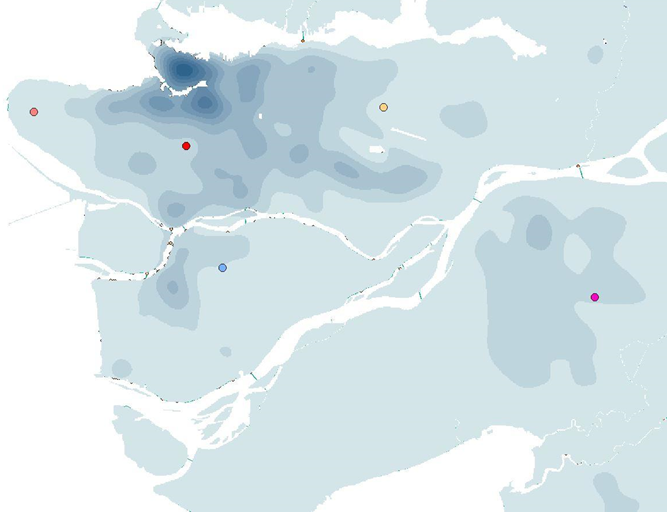
Figure 3. A raster layer of the cost surface
VI. Creating Shortest/Cost Path:
Finally, with the cost distance surface layer, we were now able to make a path that outlined the shortest distance from our arbitrarily selected point in each of the four cities (Richmond, Vancouver, Surrey and Burnaby) to the UBC campus. Taking into account the ICBC data on car crash severity and frequency around the Lower Mainland, these four paths are the safest driving routes for commuters going to UBC.
Results and Discussion
The results of the project are shown below in figure 4. Or, the map can be downloaded as a pdf by clicking here.
Based on the kernel density mapping of the ICBC crash data, all of the routes to the four residential areas head south and then east due to the high density of accidents northward of UBC. From looking at the routes, it can be estimated that there is a correlation between high density traffic areas and accidents. The routes tend to avoid major roadways in the municipalities whenever possible and veer towards less dense networks. Thus, it could be possible that main roads are more prone to accidents because of the higher volume of drivers using them. The routes outlined by the analysis is potentially a longer route from UBC to the destination in either Burnaby, Richmond, Surrey or Vancouver. This is because the analysis uses the ‘least cost’ path (which was designated by the car crash severity and frequency in a specific area) and there is a much higher density of crashes north of campus around Downtown Vancouver/ Kitsilano area.
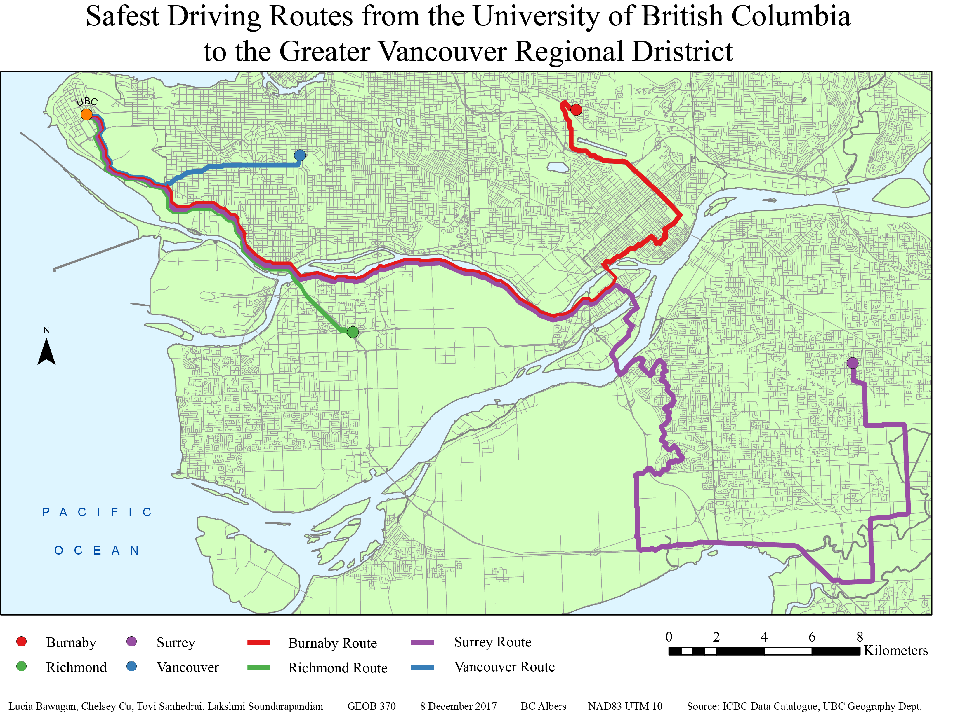
Figure 4. Final map after analysis with the four routes leading from UBC to Burnaby (red), Richmond (green), Surrey (purple) and Vancouver (blue)
Our analysis can be applied to commuter everyday life in multiple ways. It can increase the awareness of the safest driving routes between the UBC campus and the different cities in the Lower Mainland. For instance, given this information, drivers can be proactively be more alert and cautious when passing by the areas that are prone to accidents. This will encourage overall safer driving practices within the GVRD. Drivers can also avoid these areas whenever possible in order to minimize their commute times.
We would like to acknowledge that there are also points where our analysis falls short. For one, the point destinations were arbitrarily chosen rather than based on statistical analysis of which neighbourhoods most commuters are from. Furthermore, the classification of crash counts and risk levels were also arbitrarily chosen. In addition to this, there are also infinite combinations of cost by type and count when creating the ‘sum of the cost’ attribute. These errors and uncertainties could create uncertainties in our analysis and leave room for future improvements.
Further Studies
This research has been limited in scope due to the constraints in the data that we obtained. For future work, researchers could partner with the University of British Columbia to try and obtain data of where most of the university staff and students live and their mode of transportation. From there, the ones that drive to school can be singled out and an analysis can be performed based on the approximate areas which people commute to campus from. Then the analysis of the least cost path can be improved by using those areas rather areas rather than arbitrarily selecting city points.
Another step to change our analysis process would have been to normalize the ICBC data that was obtained. In our analysis we only added together the number of car crashes and the type of car crash, but it would be interesting to map out the more serious car crashes in an area over the total car crash number in the area. This would, for instance, show intersections with multiple small crashes being less dangerous than an intersection with less crashes that are more severe, informing users to avoid the latter.
Furthermore, the monitoring of accident-prone areas can help to determine how this will increase and/or shift traffic and accidents to other parts of the Greater Vancouver area. Research can also be done on whether the knowledge of the suggested routes might possibly shift the accident locations from their original locations to along the routes suggested as more and more people use these paths.
The research can also be combined with other fields such as environmental impact assessments. Investigations could occur as to whether avoiding these routes impact other areas long term. For instance, if taking these routes cause people to be caught more often in stand-still traffic due to car accidents and this, in turn, affects the amount gasoline consumed and the amount of fuel emitted into the atmosphere.
REFERENCES
ICBC Data Catalogue: http://www.icbc.com/about-icbc/newsroom/Documents/quick-statistics.pdf
- Average annual car crash data published January 2017 for the past year
- Metadata includes: crash statistics charts and accident reports
UBC Geography Department: G Drive
- Basemap: Lower Mainland Shapefile
- Road Networks: Intersection density, All roads in GVRD
- Vancouver DEM: Differentiate between road features (degree of steepness, shape of the road)
All projected in BC Albers, NAD83 UTM 10
Acknowledgments: Brian Klinkenberg and Alexander Mitchell