Abstract
Remote sensing has been prominent in monitoring the growth of urbanized areas. In the expanding city of Edmonton, Landsat data plays a key role in determining the land cover types that dominate. Through both supervised and unsupervised classifications, as well as accuracy assessments, images can be analyzed by parsing through bands and pixel values. With this information, the region can be classified to aid in future city planning projects. The results in the analysis will emphasize which method of classification is best suited to determine land cover. It is also important to note that while some land cover types are easily identified, others are not, creating a source of error. Nevertheless, this image analysis has successfully determined a general idea of land cover in Edmonton through classification.
I. Introduction
The image acquired was from Landsat 8 Operational Land Imager (OLI). This image was originally taken in 16 bit with 30 meter pixel resolution on 16 August 2016. The sensor captures multispectral images in 11 bands ranging in wavelength from 0.435 to 12.51 micrometers. For the purposes of this study, bands 1 – 7 are used. These include the visible spectrum (bands 2, 3, and 4) near infrared (band 5) and shortwave infrared (bands 6 and 7). The Landsat satellite takes a total of 16 days to circle the globe, meaning that images of one location are taken in 16 day intervals.
The area covered in Figure 1 is the northern half of the city of Edmonton, Alberta. The path number is 42 while the row is 23. The image includes part of the downtown core as well as the more suburban areas. Some of the distinct features of the area is the Canadian Forces Base as well as several golf courses. The area of study also incorporates the agricultural lands that surround the outskirts of the city. Several water features that are incorporated into the area include: the North Saskatchewan River, which slinks along the bottom right corner of the image; and Big Lake, which is located on the mid-left portion of the image.

Figure 1. True colour image of northern Edmonton, Alberta in August, 2016.
For this image, the bands were converted to 8 bit for analysis purposes. Figure 1 was created by using a combination of bands 4, 3, and 2 in order to produce a true colour image. Figure 2 is a false colour image that was created using bands 7, 5, and 3. This particular band combination shows a distinct contrast between urban areas (shown in purple and grey), water bodies (shown as blue-black), and vegetation (appearing as green). In using this, certain key features are easier to identify.

Figure 2. False colour image of northern Edmonton, Alberta in August, 2016.
In comparing the Landsat OLI imagery to the ESRI basemap imagery, one can tell from the colouring of the image, which was taken at an earlier date. The Landsat imagery has more greenery since it was taken in the summer. The basemap appears to have more barren land indicating that it has been taken around late winter to early spring. The image acquired also shows some sites that are different from the basemap. For instance, some areas that are under construction or buildings that were not previously erected appear in the basemap while not in the 2016 image. Since the ESRI basemaps are regularly update, this would mean that the basemap is the most up-to-date version of the study area. And in fact, the basemap image was taken on 14 March 2018, making it more recent than the 2016 image that was obtained for analysis.
II. Analysis
Image classification extracts information from the classes of a multiband raster image. There are two types of classifications: supervised and unsupervised, which vary depending on how the analyst uses the software. In supervised classification, spectral signatures are obtained from training samples that the analyst creates to classify an image. For unsupervised classification, the software finds spectral classes (also known as clusters) in a multiband image without intervention from the analyst.
A. Unsupervised Classification
As part of the analysis, an ISO cluster unsupervised classification was performed using all of the available bands, classifying the image into 50 classes. From there a dendrogram was produced, which grouped together the most similar classes from the results of the ISO classification. This made it easier to identify the best way to further narrow down the classes. Based on the dendrogram, the 50 classes were grouped into 6 different categories: water, commercial/residential, dry grass, trees, agricultural, and industrial. Table 1 shows the number of pixels that are incorporated into each category. Since the pixel size for the image was 30 meters by 30 meters, in order to determine how many hectares that translated to, pixel counts in their respective categories was multiplied by 900 meters squared and then converted into hectares.

Table 1. Values of ISO cluster unsupervised classification of northern Edmonton. Class Pixel
The unsupervised classification procedure was able to produce fairly accurate results. The results are shown below in Figure 3. The most distinct class was water, as the pixel value did not match up with any other class. It was hard to identify tree cover areas because the dendrogram grouped those values together with the rest of the grass fields. This could have left substantial room for error as these pixel values then had to be manually reclassified by the analyst. But after shifting around some of the reclassified values, the grass fields that were classified under agricultural land, become distinct features. Also, it is notable that areas of barren soil or dry grass are easily confused with industrial regions because of the similar pixel values. The program further had difficulties in differentiating between the different land use types in the urban sprawl. This is understandable, since unsupervised classification is best used for land cover identification, not land use.
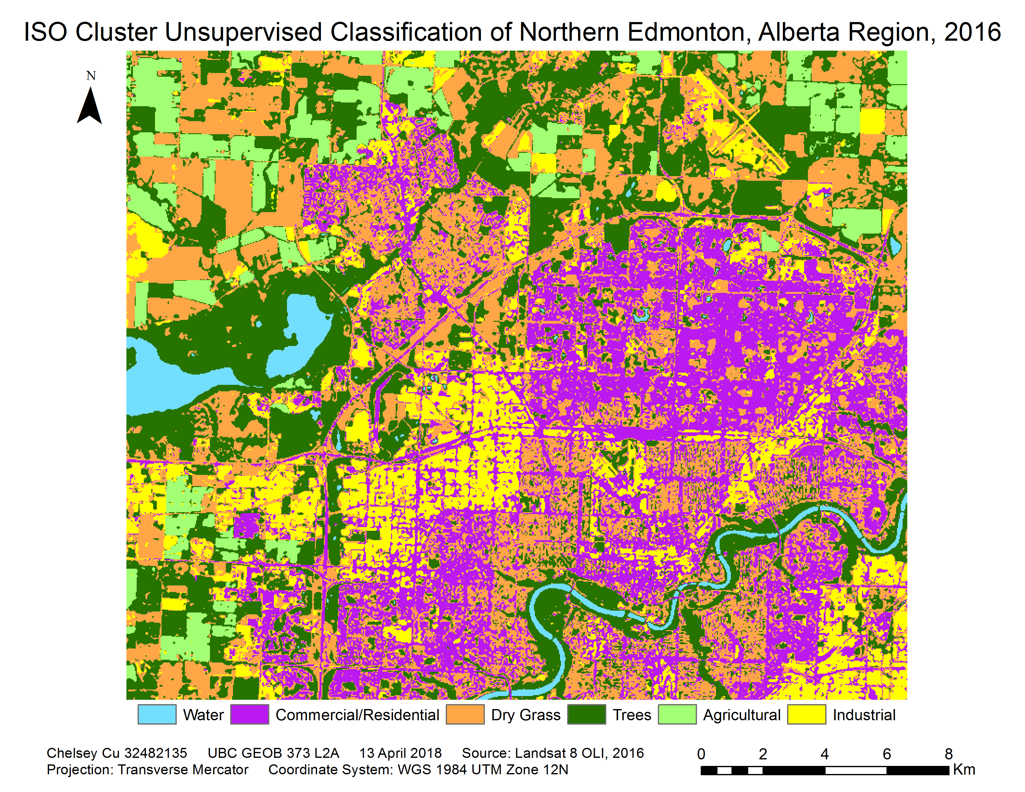
Figure 3. ISO cluster unsupervised classification with a majority 8 filter of northern Edmonton, Alberta in August, 2016.
B. Supervised Classification
Following the unsupervised classification, a supervised classification was performed. Here, training sites were created, using the results from the unsupervised classification as a guideline (see Figure 4). Several training sites were created for each of the previously delineated regions. This increases the accuracy of the analyst-made training sites by pinpointing areas that have previously been grouped together by the software. From these training sites, histograms (see Figure 5), and scatter plots (see Figure 6) can be made from the pixel statistics (see Appendix A). Finally, with the signature files created from the training sites, a Maximum Likelihood classification (MLC) and an accompanying output confidence raster (OCR) was produced.

Figure 4. Training sample sites for supervised classification of Edmonton, Alberta, 2016.
The Maximum Likelihood classification places pixels in a class based on the probability of a pixel belonging to a class. Both the variance and the covariance of the class signatures are considered to determine which cells belong to which classes. The output confidence raster is a means to determine the accuracy of the MLC results. Values are assigned to each pixel based on the software’s certainty that it was classified correctly. A value of 1 to 14 is then assigned each pixel with the lowest values representing the areas with the highest reliability.

Figure 5. Histograms of the analyst-created training sites showing the separability of classes.

Figure 6. Scattergram of the analyst-created training sites showing the separability of classes.
Looking at Figure 5 and 6, the spectral separability of the classes appear to be quite low. Most of the bars as well as the points of different classes seem to overlap in both images. This is problematic because it means that there is a higher chance that objects in the image were misclassified, thus decreasing the accuracy of the results. The best results are if the different classes are in distinct clusters. This helps when the program is classifying pixels that have not been incorporated into training samples. It enables the program to determine exactly what class a random pixel should be placed upon based on its spectral value. However, since the spectral separability in this case is seems to overlap between classes on all 7 planes, the pixel classification could be inaccurate as a pixel that has been classified into one category, could just as easily have been misclassified into another based on its value. For instance, when consulting Appendix A, it can be noted that classes such as agriculture and water are the most accurate, while industrial areas are seen as the least accurate. This could mean that pixel values for industrial areas can be easily misinterpreted and placed into other categories. In fact, this was seen in the unsupervised classification, when multiple dry grass areas were misclassified as industrial.
The results of the supervised and unsupervised classification can initially be compared though looking at Figure 3 and 7. In both cases, a majority 8 filter done on the final image to try to reduce fragmentation. The filter put pixels into the same category as its eight nearest neighbours. In Figure 3, there is a lot more fragmentation between land use classes. Therefore, the image ends up looking patchy, especially in the commercial/residential and industrial areas. While classification may be more accurate, it is also harder to interpret. In Figure 7, one can immediately notice that there is a lot more cohesion in the commercial/residential and industrial areas. Through the training areas that were made (see Figure 4), larger areas that previously had different ISO classes were placed into the same category. In some ways, this classification is less accurate, because large areas are clumped together into one category, meaning smaller scale data might be lost. But it also provides more cohesion between areas allowing the map user to clearly identify areas that each class occupies. Further, since it was a supervised classification, some of the areas that were previously misclassified in Figure 3 was corrected by creating training areas on those locations and manually classifying them into the correct category. In this way, the MLC was able to correct the classification errors produced during the unsupervised classification.

Figure 7. Resulting Maximum Likelihood from a supervised classification with a majority 8 filter of northern Edmonton, Alberta in August, 2016.

Figure 8. Resulting output confidence raster of the Maximum Likelihood from a supervised classification of northern Edmonton, Alberta in August, 2016.

Table 2. Values of Maximum Likelihood supervised classification of northern Edmonton.
Similar to Table 1, Table 2 shows the shows the number of pixels that are incorporated into each category. These have been converted into hectares to identify how much land belongs in each field. In comparing the two tables, the values that fluctuate the most are dry grass. This confirms the earlier speculation that many of the dry grass areas were inaccurately classified as industrial regions. The agricultural areas changed the least, showing that those areas are the most accurately classified in both cases.
Based on the output confidence raster of the MLC does not seem to be very accurate. In Figure 8, there are very few patches of green and quite a large number of pixels that are red, showing that only a small area was reliably classified. The most concerning red region is the North Saskatchewan River. In the unsupervised classification, water was identified as having a dissimilar pixel value to all the others, classification of waterbodies the most accurate. In the supervised classification results, the river is identified as being poorly classified. Moreover, the large amounts of yellow identified in the OCR shows the lack of ability of the supervised classification to accurately identify land cover types.
C. Accuracy Assessment
The pseudo accuracy assessment compares the supervised classified image to the unsupervised classification of the image. In this case, the ISO cluster unsupervised classification results are considered “accurate” or the ground truth data. This is compared to the MLC results to see how accurate the classification was for each of the classes. The row at the top of the chart is the labels from the supervised classification while the left-most columns are show labels from the unsupervised classification. The values that have been bolded in black are the ones that are used to determine accuracy. Based on the assessment, the ISO classes that are the most accurately classified are Trees and Commercial/Residential areas, the one that is the least accurately classified is water. Kappa evaluates how well the classification was performed in comparison to jut randomized values. The value for Kappa is 0.579. This is verified with the percent of the image that is correctly classified at 66.8 percent.
III. Conclusion
Overall, based on the results of the pseudo accuracy assessment, the supervised and unsupervised classification, this seems to be fairly inaccurate. The pseudo accuracy results indicated that with the unsupervised classification, only about 67 percent of the image was correctly classified in comparison to the ground truth data from the unsupervised classification. Looking at the results, classes such as water, which have distinct pixel values, are more accurately classified, while industrial areas have a lower accuracy.
Given the results, the best classification route for identifying land cover would be unsupervised. While land use would be best identified using supervised classification. Land cover can be identified by the pixel values that the sensor records; it consists of only physical characteristics. Land use is more of a social aspect and cannot be as easily identified based on a software and pixel values. For instance, the land cover could be vegetation, but the land use could be agricultural, gold courses or sports fields. Therefore, land use depends more on user classification and cannot be accurately done by the software. Overall, land cover classification can be improved through more information. The spectral separability is key for accuracy, and while there will always be human error created from the analyst, better image quality from improved sensors will help to eliminate this. As spectral separability becomes more accurate, unsupervised classification will as well.