Define study area:
Study area has been selected based on following criteria:
- Area with high tree coverage (based on observation form Google Earth);
- Tree shadow will influence nearby houses;
- Tree fall could cause potential damage to nearby houses.
After applying all the condition, a study area at the North of Dunbar community and around Balaclava Park. This study will mainly focus on houses at Blenheim Street. This area has a size around 0.3 km2 (based on google earth measurement).
Tree Shadow Analysis
Tree DEM
The raw LiDAR data in LAS format was converted to LAS dataset. And projection was added for it to be readable by ArcGIS. Then, the tree data was generated and converted to DEM data by filtering the LAS dataset using return value of 3, which represents lower vegetation (trees that are shorter than 8m) and return value of 5 which represents high vegetation (trees that are taller than 8m). Also, ground DEM data was generated and converted from LAS dataset using return value of 2. Each cell size was set to 1.5 meters. In order to obtain the height and crown size of trees, the ground layer was subtracted from the tree layer, and the new data is the DEM of tree that I will be working on later.
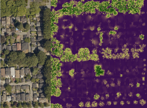
Figure 1. The DEM (right) containing tree height and crown size compared with real-world (left) data to ensure accuracy.
Tree shadow analysis
The shadow on the ground can be calculated using a DEM and hillshade tool (Li et. al., 2005). When conduct shadow analysis, three factors should be considered: sun’s position, tree’s crown size and tree species. The first one is the sun’s position. The shadow is caused by trees blocking sunlight at certain sun altitude and azimuth. Since the earth has a tilt axis and is rotating around the sun, the sun altitude and azimuth will change rapidly. Therefore, a specific time should be determined to get precise altitude and azimuth value that will be used in hillshade calculation. The second factor is the tree’s crown size. The crown size is different in each season due presence of leaves. In the summer, the canopy coverage is at the maximum value, and in the winter, the canopy coverage is at the minimum value. Thus, two analyses, summer and winter, should be made to show the seasonal difference. The third factor is the tree species. As we know, only deciduous tree species will shed its leaves in fall. Therefore, the tree species in this study area should be cross-check with the street tree attribute to ensure its crown size in winter.
Next, two specific date and time of July 9th, 2013 at 11 a.m. and Nov 19th, 2013 at 11 a.m. were selected to present summer and winter influence. On July 9th, 2019, the sun has an altitude of 52.23 degree and azimuth of 123.19 degree, and on Nov 19th, 2019, the sun has an altitude of 20.20 degree and azimuth of 166.25 degree (SunCalc, 2019). and all the trees in this study area has been confirmed to be deciduous species.
The hillshade functions with corresponding input altitude value and input azimuth value were applied to tree DEM. The results were called “summer shade” and “winter shade” respectively.
Then, the results were reclassified into 2 categories, light and shade. In the result of “summer shade”, all cells with values that are greater than 1 were reclassified to 1 (ArcGIS Help). The winter break value was set to contain less of the cells than summer, since the tree do not have leaves during winter.
a) 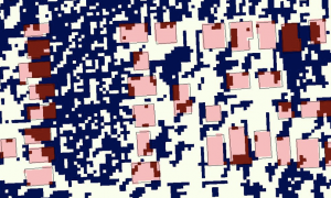
b)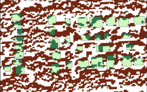
Figure 2. The hillshade calculation result (partial map). Summer shade coverage on the top (a), and the winter shade coverage on the bottom (b). In a), the dark red indicates the shadow on each building, the light red indicates that the sunlight will not be blocked by trees. The background of the dark blue points is the reclassified hillshade result. In b), the dark green indicates the shadow on each building, the light green indicates that the sunlight will not be blocked by trees. The background of the dark red points is the reclassified hillshade result.
Fallen Tree Damage
Tree height calculation
There are two obstacles with the tree height data sets. First, the street tree data found from Vancouver open data catalogue only recorded the tree height in height range class (i.e. 0-10 for every 10 feet, such as 0 = 0-10 ft, 1 = 10-20 ft, 2 = 20-30 ft, and 10 = 100+ ft) , which is not accurate for the following analysis. Second, trees are continuously growing every year. Therefore, in order to analyze the current influence of the tree, the height of each tree should be corrected. A tree guide was consulted to find the average growth rate of each species presented in the study area. The growth rate of each species was summarized as follows:
| Genus Name | Species Name | Common Name | Growth Rate (cm/y) | Mature Size (m) |
| Acer | Platanoides | Norway Maple | 45 | 22 |
| Quercus | Coccinea | Scarlet Oak | 40 | 22 |
| Quercus | Palustris | Pin Oak | 40 | 24 |
| Quercus | Rubra | Red Oak | 40 | 23 |
| Fraxinus | Pennsylvanica | Bergeson Ash | 60 | 18 |
| Fraxinus | Ornus | Flowering Ash | 50 | 18 |
| Ulmus | Americana | American Elm | 78 | 19 |
| Ulmus | Pumila | Siberian Elm | 70 | 19 |
| Ulmus | Glabra | Scots Elm | 75 | 19 |
| Fagus | Sylvatica | Golden Dawyck Beech | 45 | 18 |
| Betula | Pendula | European White Birch | 60 | 21 |
| Prunus | Cerasifera | Pissard Plum | 35 | 8 |
| Prunus | Serrulata | Pink Perfection Cherry | 35 | 8 |
(Find Trees – Tree Guide, 2019; E-Flora BC, 2019)
The current height of each tree was calculated using field calculator and applying formula: Current Height = (height range id) *304.8+3 years*annual growth rate, then the results of current height of each tree were adjusted manually to make sure that it did not go above the mature height, which is the maximum size of each tree.
Fallen direction analysis
Firstly, the damage range of each tree were plotted by applying buffer of each tree’s current height, this provided a maximum range that can be influenced by a fallen tree.
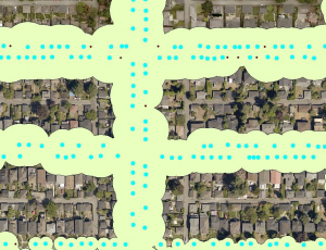
Figure 3. the potential damage area of each fallen tree. The blue points indicate each big tree’s location. The red points indicate each small tree’s (less than 4m) location, since their height are too short and crown sizes are too small, no buffer is applied to them. The yellow region indicates the potential damage area.
Then, Euclidean direction function was applied to each tree to get its fallen direction. However, the Euclidean direction only provide output value based on compass direction, and in real life the tree always falls to downwind direction (Rentch, 2010). Thus, this analysis used the wind data of Oct 25th, 2019 to predict damage. According to Vancouver historical Wind Direction, on Oct 25th, 2019, the strongest wind was blowing at 270° at a speed of 76 km/h (Vancouver Historical Wind Speed, 2019) and this wind is strong enough to cause damage. Finally, reclassify and recolour the fallen direction according to wind direction.
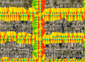
Figure 4. The falling direction of each street tree. Red indicates the most possible falling direction, yellow indicates the less possible falling direction, and the green indicates the impossible falling direction.
Damage on each nearby house
To study the damage on each nearby house, using the falling direction data form pervious step and then “extract by mask” to find the potential damage on each nearby house.
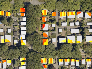
Figure 5. the potential fallen tree damage on each nearby house on Oct. 25th, 2019. Red indicates a high possibility of being damaged, yellow indicates a fair possibility of being damaged, and grey indicate a low possibility of being damaged.