Figure 3. Map representation of kriging interpolation result
Kriging is used on spatially correlated samples. Interpolation results use spatial autocorrelation to assign weights used to predict value at an unknown location. A “Simple” kriging type is used, and second order polynomial trend is removed through the detrending step. For all following steps, the “Optimize Model” tool is used to find the appropriate settings that yielded the lowest root mean square error. During the neighborhood step, maximum neighbors are set to 5 due to the low sample size and sector type is set to 8. In the cross-validation step, a mean standardized error of -0.12 are given (value should be close to 0) and a root mean square standardized error of 1.58 is yielded (optimally should be close to 1). This shows the model is underestimating the variability in the predictions.
After restoring the DALR, the final kriging result clearly shows the temperature variation with elevation. It also shows a more representation of West-East temperature variation since interior BC is warmer in summer than coastal cities. However, it does not seem very accurate as the temperature change should occur further away from the coast.
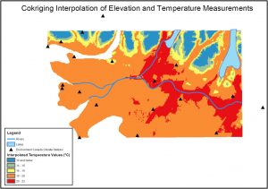
Figure 4. Map representation of cokriging interpolation result
The process is similar to kriging instead two variables are used for interpolation instead of one. The two variables used are the elevation value extracted from the DEM and the uncorrected mean temperature measured at stations. During the cross-validation step, a root mean square standard error of 0.9 is given to the model. In the cross-validation step, a mean standardized error of -0.06 are given (value should be close to 0), and a root mean square standardized error of 0.9 is yielded (optimally should be close to 1). The error value shows the model is overestimating the variability in the predictions.
The final cokriging result map shows the temperature variation with elevation. Surprisingly it also shows a more accurate representation of West-East temperature variation.
Figure 5. Map representation of Inverse distance weighted interpolation result
Inverse distance weighted is a deterministic method of interpolation. IDW interpolates relative to prediction location; closer known sample points are weighted “heavier” than known sample points further away when interpolating. In the cross-validation step, a root mean square error of 2.02 is yielded (optimally should be close to 0). The error shows the model is overestimating in its prediction and is off by 2 °C.
After restoring the DALR, the final result map looks reasonable and shows the temperature variation with elevation. However, west-east temperature variations are not apparent.


