
It’s a nightmare scenario to modern science students: facing a physics midterm with a dead calculator. We have all used these miniature computers so extensively in learning math that most of us don’t trust ourselves to do it any other way.
We are all aware that there must have been some stygian era before these wonderful devices came into existence. Calculations must all have been carried out manually. This is not the case. Before there were digital computers, there were analog computers.
The first known analog computer was manufactured around 100 BC. This device, known as the Antikythera mechanism, was used by ancient Greek astronomers to predict the movement of celestial bodies.
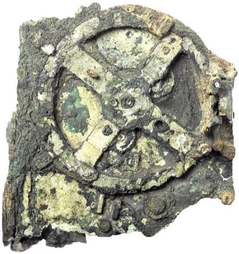
A fragment of the Antikythera mechanism. Source: computus.org
Analog computers reached their most advanced forms in the 1950s, when they were used in to aim the weapons of naval vessels. This may seem counter-intuitive; artillery problems are used to teach some of the simplest concepts in first-year physics, surely this could be done by hand. Bear in mind, these simple artillery problems have only two dimensions and involve stationary targets and stationary firing platforms all operating in a frictionless vacuum.
The real world is so much more complex than these problems that fire-control computers accepted as many as 25 variables. For comparison, the simplest kinematics problems have 5 variables. A mathematician could do the same calculation in minutes, at best, and only then for one selected instant. Fire-control required continuous output under constantly changing conditions.
While the history of these devices is interesting, how do they work? To illustrate the basic principle, we’ll construct a very simple analog computer.
For illustrative purposes, our goal will be simple, to divide by two. We will call our known, or input, variable y and our unknown, or output, x. The function calculated is:
y=2x
To start we have two wheels, which could just as easily be gears, designated A and B.

Public domain
Wheel A has a diameter of 1, wheel B has a diameter of 2. Since circumference is the diameter multiplied by pi, if the outside edge of A were flattened out, it would be half the length of the similarly flattened edge of B. When A turns once, it will roll along half the edge of B, driving a half revolution of B.

Public domain
The revolutions of A represent the input and the revolutions of B represent the output. Six turns of A will produce three turns of B, just as 6/2=3.
To make input and the reading of output easier, we can label the inputs and outputs on the wheels. For simplicity, only a few outputs are labelled, but high resolution can be achieved with the same principle.
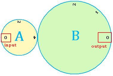
Public domain
Here, we see that the input and, consequently, the output, are zero. Rotating A 90 degrees, rotates B 45, so that the input of 2, gives an output of 1.
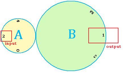
Public domain
Analog computers have many more complex mechanisms, but the guiding principle is the same; displacement or rotation of components used to model variable values.
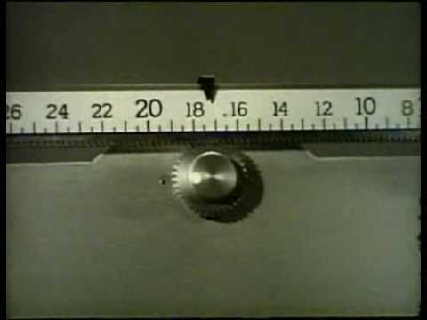
This 6 part training film outlines this and many more mechanisms used in mechanical computers.
References
(1) The Antikythera Mechanism Project The Antikythera Mechanism Project. http://www.antikythera-mechanism.gr/ (accessed 02/12, 2012).
(2) Navy Dept. Bureau of Ordnance In Basic Fire Control Mechanisms; Ford Instrument Co. Inc.: Long Island City, NY, 1944; , pp 425.
2 responses to “Doing It The Old Fashioned Way”