Weebly website: https://issuesinbcpubliclibraries.weebly.com/ 

 

Objectives

Our objective for this project  was to create a website with accompanying data visualizations and infographic elements that would provide a broad  indication of trends in various issues concerning B.C. public libraries and Canadian public libraries in general. We chose to include issues surrounding overall  funding for public libraries, the rise of precarious employment among librarians and library staff, and the issues public libraries face  concerning e-books and other e-content. We also included some reported material on the effect Covid-19 has had on these trends.

 

Data

We previously had a different topic and direction for this project, but unfortunately the saying “biting off more than you can chew” applies here. We found that the available data for the proposed project was far too large and unwieldy, so we decided to pursue a different topic in a related field. The data we access for this final project was collected by the B.C. provincial government and it contains 16 years of data reported by B.C. libraries. 

The original format of the data was in several sheets in a combined Excel workbook. There was no questionnaire key available on the B.C. website’s for this data (https://catalogue.data.gov.bc.ca/dataset/bc-public-libraries-statistics-2002-present), that information as only available in the frozen top row of each sheet, and as the questions for each year changed as some field were retired and new ones were added, it was difficult to compile the data into a Tableau-friendly sheet which keeping track of all of them. The final combined Excel file contained 242 columns of data for roughly 70 B.C. library systems over 16 years. The reporting was patchy in some places and some failed calculations appeared in others, still there is plenty of consistent data, especially concerning finances. Minor issues were mostly resolved in Tableau, for some visualizations we created curated Excel files of only the data we wished to use in Tableau.

 

Visualizations

The visualizations we created were from data over several years and benefited the design aspect to use line charts to show the financial data. In this design we used the basic design elements available in Tableau and did not “mess with it”, “it” being the standard formatting for visualizations in tableau. Since the basic formatting for Tableau visualizations is soft, not harsh on the eyes, and is very direct it matched well with both the design of our Weebly website and the infographic materials we produced with Piktochart. 

 

News Sources

Both before and after creating the visualizations, we consulted online articles from reputable sources (mostly the various provincial specific reports for CBC news, lots of library drama happening in Newfoundland) for information to apply to the creation of our project. We incorporated a lot of this information into the infographic materials and it informed us in the creation of our visualizations in Tableau, specifically in cherry picking what data to use from the massive amount of data that we cleaned.

 

Infographic materials

The infographic materials we created for this project were produced using Piktochart. While there are many infographic templates available on Piktochart, we did not directly apply a template to our project, instead choosing a template to delete most of its elements and work from the ground up. Since we were creating graphics for a website rather than a purely a stand alone infographic we made the graphics much larger (2000 px width) to compensate for the width of the website. We also created the infographic with the intent of “breaking it up” into individual panels interspersed with data visualizations from tableau. It was not made to be viewed as one solid infographic (and if you tried to do that it would honestly look kind of ugly). The overall design of the infographic materials favors soft textures with a blue and grey color palette. The only time blue and grey are not used are for impact, or when they cannot be applicable to certain graphics. Piktochart already has some great face-masked illustrations that we incorporated into a recurring section at the bottom of each infographic segment.

 

Website

We decided to create a website through Weebly as a much easier route for compiling all the parts of the final project, which includes a slideshow of static visualizations and the compiled information from several news stories on the subject in infographic form. Weebly was fairly easy to use for a free online tool and any drawbacks we might have encountered did not unduly hinder us.

Our dashboard can be found here.

Our infographics can be found here.

Introduction

In this project, we designed an interactive dashboard that enables the audience to explore the relationship between the characteristics of a medical insurance beneficiary, such as age, Body Mass Index (BMI), smoking status, and the insurance costs incurred in the United States. By visualizing the Medical Cost Personal Dataset, we try to answer questions such as does an increasing BMI increase the medical costs? How about age? Number of children? Smoking status? Furthermore, we designed infographics to demonstrate our findings in the correlation between personal factors and medical costs.

Our intended audience is the public that is interested in medical expenses. The US is well-known for its lack of universal healthcare and perplexing health insurances. We hope our design could help the audience make informed decisions with regard to healthier lifestyles, no matter if they have the privilege to visit hospitals.

Data

For this project, we are using the Medical Cost Personal Dataset. This dataset is used in the book Machine Learning with R by Brett Lantz and extracted from Kaggle by Github user @meperezcuello. The data is in the public domain. (meperezcuello, 2019) Originally, the dataset was used to train a machine learning model to predict the insurance cost. We are aware that it is only a small sample of medical insurance costs in the US of people aging from 18 – 64. There’s no detailed demographic information such as race and county. And it cannot reflect the health condition of people who don’t have insurance.

It has 7 attributes and 1338 records. The attributes are as follows:

Tools

For the interactive dashboard, we use the Tableau Desktop. Tableau is very easy to use when doing visual analytics. Compared with Shiny or Plotly, Tableau requires minimal technology shrewdness to build a dashboard. It also provides a variety of native visualization idioms and color palettes that are sufficient for our project. Another reason we choose Tableau is that it provides a free platform where we can easily publish our work. For the infographics, we used infogram. It was a great tool to use because it had lots of templates which are easy to modify. And it’s also user friendly.

Analysis

We first made some static visualizations to get familiar with the data and understand the distribution. The dataset has most samples in the 18 – 25 age group. The largest difference of numbers of beneficiaries from both sexes is also in this age group.

The distribution of insurance charges is right skewed. More than half of the charges are lower than 12,000. A few records are higher than 50,000.

On average, male beneficiaries are charged more than female ones. The difference is more drastic across different age groups and smoking status.

We once thought the number of children covered by insurance may also be a factor that affects the charges. But the following box plot shows that the medians of charges across different numbers of children are quite close to each other. The distribution of charges of beneficiaries having no minor dependents is wider than other beneficiary groups. The most expensive charges also show up in this group. The minimum of charges grows steadily when there are more children covered by insurance. But there’s no clear pattern of the maximum. One possible explanation is that people who have no minor dependents may be older and have independent grown-up kids. Therefore they may have more medical costs due to their age.

We used two scatter plots to discover the relationship between quantitative variables, namely age vs. charges, and BMI vs. charges.

The scatter plot on the left hand side indicates the relationship between BMI and medical charges. There’s no clear pattern in the graph. The plot on the right hand side shows the relationship between age and charges. There are three clusters with similar slopes, growing as the age increases. When we take sex and smoking status into concern, it shows that there’s no clear difference in distribution between sexes, while the smoking status tells us more interesting information.

The BMI-vs-charges graph implies a positive correlation between BMI and medical charges within smokers. The age-vs-chages graph shows that smokers dominate the highest cluster, non smokers the lowest. These two graphs are later used in the interactive dashboard.

Design Approach

We developed our design approach by analyzing our target audience’s tasks. We aim to allow users to play with the data and find out the relationship between medical costs and factors of their choice, such as age, gender, and region. Using Munzner’s framework of task abstraction, we identify our audience’s goal at the highest level is to discover the relationship between medical costs and other factors. At the lower level, our design should allow users to compare between different groups, such as age, sex, and region. Due to the simplicity of our data (only 7 attributes and 1338 records) and the lack of granularity, our design doesn’t emphasize the mid-level tasks such as looking up and locating.

To support discovery of the relationship between quantitative variables, we designed a scatter plot where users can choose the x-axis. The y-axis is fixed and indicates the medical costs. Furthermore, to support the visual queries of comparing groups of data, such as male vs. female, and smoker vs. non-smoker, we used a pre-attentive visual primitive, namely colors (Ware, p.29). When choosing “breakdown by sex” or “breakdown by smoking status”, the spots will be divided into two colors. When breaking down by sex, it is difficult to separate the two colors, which indicate male and female, from each other. On the other hand, when breaking down by smoking status, the red spots indicating smokers pop up and show a clear trend different from the green spots, which indicates non-smokers.

The principle of soundness/utility/attractiveness were used in the design. The infographics gives a detailed overview of the factors that affect medical cost in the Northwest, Northeast, Southwest and Southeast region of the United States. It shows the Sex and number of records for each age group. It also shows how age and lifestyle (smoking) plays a factor in medical cost. All information in the infographics are truthful and honest. The data representation and credible analysis was gotten from Medical Cost Personal Dataset. Simple illustrations were used which complements the data conveyed in the infographic. Being a medical related topic, white was used as the background colour as it is associated with medicine/hospital. For the age factor, bold colours were used for the younger age range as it signifies strength and agility that comes with young age while warm colours were used for the older age range as it signifies security. Furthermore, two font sizes were used, one for heading and subheading while the other for body. All texts were aligned evenly. Overall, infogram was a great tool to use expect for one or two challenges we had- we found it difficult to customise the pictogram template to our desired choice.

Reference

Meperezcuello. (2019). Medical Cost Personal Dataset. Retrieved from https://gist.github.com/meperezcuello/82a9f1c1c473d6585e750ad2e3c05a41#file-readme-md.
Munzner, T. (2014). Visualization analysis and design. Boca Raton: CRC Press.
Ware, C. (2008). Visual thinking for design. Burlington, MA: Morgan Kaufmann.

Link to Website: https://northarmfraser.weebly.com/

The Story

The story I am telling with my website is that the place names along the North Arm Fraser River reflect the British colonial legacy, but do not adequately reflect the people who live here and who have lived here. The most names refer to white, British men, and only six names refer to Indigenous peoples or women. My website questions how the names were given, who is left out, and how likely it is for names to change.

 

Objectives

The main goals of this project are to inform viewers about the colonial legacy in place names along the North Arm Fraser River and to entertain viewers by letting them discover the history of names. Viewers are able to explore place names and their histories and compare the origins of various names. Users are also able to filter and select data, and consume the information. These tasks are both high level and low level. In making the visualization, I produced new knowledge – I had hypotheses about what the data would show, but no one I know of has done a similar analysis along the North Arm Fraser River.

 

Dataset Details

The dataset I used includes the names of places along the North Arm Fraser River and categorizations of what the names refer to. I collected and categorized the names myself using three sets of maps: Google Earth, North Arm Fraser River Harbour Head Line Maps from 1965-1967 (Underhill & Underhill 1965-7), and the Sto:lo-Coast Salish Historical Atlas (Carlson et al. 2001). I chose these three sources because Google’s platform is commonly used by the public for navigation and remote exploration, and it shows names the public is most likely to be familiar with. The harbour maps add a historical perspective, showing places where names have changed or streets have been altered. These were paper maps that happened to be in an appendix to a past student’s thesis, which I picked up at the library before campus closed (Figure 1). Finally, because of the lack of indigenous names in the other datasets and my desire to emphasize that this is Indigenous land, I included names from the Sto:lo-Coast Salish Historical Atlas.

Figure 1. Collecting names from the harbour maps.

Most of the maps I viewed were not specific to the river and contained names across Metro Vancouver. For this project, I limited the names I collected to those that described the water (ie inlets, jetties, sloughs), described the shore (parks, neighborhoods), and named streets that ended at the shoreline or traversed the shoreline. Collecting names in Google Earth was most challenging, because different names appeared depending on the level of zoom I used.

I organized the names into eight categories with the help of the Greater Vancouver Book, Street Names of Vancouver, the City of Richmond Archives place names search, and Google searches (citations for these resources can be found at the bottom of the website I created). When the names referred to people, I collected more information, including gender, race, year of birth, and notable facts. I was sometimes unable to find the history of a place name or information about the person. Such names were added to an unknown category, which is visible on the map and in the bar charts. Some people were repeated in names and excluded repeats in my demographic analyses. Part of this spreadsheet can be seen in Figure 2.

Figure 2. My Excel spreadsheet.

Tools

As I collected place names, I georeferenced them using Google Earth Pro. This program let me mark points on a map and name them. I then exported the points from Google Earth as a kml file. Working with the kml file was challenging because the file type cannot be opened and viewed as a spreadsheet on my computer. After I had added all my places, I was able to copy the names from the Table of Contents (a sidebar allowing the user to control layers and points) and paste the names into an Excel file, where I categorized and described the place names. This categorization required significant research into the history of Vancouver, Richmond, and New Westminster. References for the various sources I used can be found in the Bibliography section of my website. I was uncertain if joining the kml data with my Excel file would be successful, but luckily it was.

Figure 3. The Google Earth interface with my data points.

I joined the two files in Tableau Desktop, then used Tableau to create a map of my dataset and several bar charts showing trends in the data. The Tableau mapping feature allowed me to plot my points by category, highlight similar points, allow sorting by category and by source, and show information when hovering over a point. Being able to both map and run analytics in the same program was convenient. I could also have used QGIS or ArcGIS for creating a map and charts, but I am less familiar with interactivity on those mapping tools, and I don’t feel as though I have as much control over associated analytics with those tools and my current knowledge.

Once I created my visualizations, I wanted to add them to a platform where they could be combined with textual information. I chose to use Weebly website creator, because I’ve used Weebly before, I knew I could embed interactive visualizations, and I don’t like how Tableau Stories looks. I uploaded my map to Tableau public, then added embedded it in Weebly. I also embedded a map from Native Land. Weebly had themes and outlines prepared that I used, and to add extra features, I simply dragged-and-dropped. Weebly is not an open-source platform and their websites do not stay around forever – I would rather have used a different platform like Github or Jekyll, but did not have the time or energy to learn something new.

 

Analytic Steps in the Design Process

To create my website, I relied on observations that I made during data collection and patterns that appeared while mapping. As I collected names, I noticed certain patterns, such as repetitive names, lack of names relating to Indigenous peoples and women, and high representation of British patriotic symbols and British men’s names. When I began the project, I had hypothesized that names would refer mostly to white men, there would be few Indigenous names, and the names would have been given in the late 19th and early 20th century, as Vancouver grew, meaning that people would have been born in the early-mid 1800s. These hypotheses were affirmed, and new patterns, such as repetition of certain names like River Rd and Boundary Rd and a high number of British names appeared. I produced knowledge while gathering the data, albeit working from a hypothesis, and then communicated knowledge as I made my visualizations. The analytics I ran on my data, visible as bar charts on my website, were used to communicate my findings – I had already observed the patterns while inputting the data.

 

Design Process and Principles

The first visual I designed was a Tableau map, which I later embedded in Weebly. On the map, the places are color-coded and sortable by category, and they can also be sorted by source. Users can pan and zoom and use the a search bar to search for specific places names. I chose a neutral color scheme for the points that is distinct from the background and is not hierarchical. I also changed the background map to one with more color, because when I initially embedded the grey map on my website the map disappeared into the background rather than standing out as the highlight of the project. Due to the gentle colors of my website, the colors of the dots and background features on my map stand out in our pre-attentive/tunable vision. On my map, I used the highlight feature so that all points of a similar category appear when a viewer hovers over one point. I also added text on hover that gives the place name, category, and any notable information about the name. I ensured that the place name was in bold and separated from the other information, so that it would catch the viewer’s attention before the extra details. See Figure 4.

Figure 4. Place names map embedded in website.

The map is expressive because spatial data is shown using geographic coordinates and color is used to encode an identity channel. The colors chosen are not hierarchical implying a magnitude channel. The map is also effective because it communicates information using interactivity rather than flooding the viewer with information at first glance, offers various means of sorting the data, and is visually appealing.

In my bar charts, I maintained the color scheme from the map for the chart of categories, but I used the green hue from the map for the other charts. These charts can be seen in Figure 5. The consistency in color choice helps maintain unity on the website and makes the charts feel like they go together, rather than being separate visuals. To maintain expressiveness, I ensured that repeat names were not present in the data for the bar charts. The choice of bar charts was also to ensure expressiveness, because bar charts allow comparison between values without suggesting a hierarchy or that individual groupings are sections of a whole.

Figure 5. Sample bar charts.

For the color scheme of my website, I chose green and white, using the green from my map and bar charts. The green backgrounds are the green with less luminance because we learned that background colors should not be as vibrant. I maintained the darker green in my headers. Finally, the pre-created theme from Weebly had fonts that were readable and matched the semi-serious but exploratory mood of my content.

 

Pros and Cons of a Website

I chose to use a website because the format allows more text than other formats, such as infographics or stand-alone visualizations. For my story, in which I’m inviting viewers to question dominant narratives, having text to guide viewers through new ideas is essential. A website also allows for a variety of visuals, including photos and newspaper articles, to be embedded, which can break up large chunks of text.

On the other hand, websites can make a story challenging to tell, because there can be too much text and viewers can get “scroll fatigue.” In making my website, I struggled to keep my sections visually interesting so that the viewer would want to read on and continue scrolling down the page. Adding blank space and muting the colors helped with readability. Another drawback of a website is that the length of the text on my website draws away from the effort I put into my map – the map disappears into the page, rather than being highlighted as the main output of my project.

 

References

1. Carlson, K., McHalsie, A. J., & Perrier, J. (2001). A Sto:lo-Coast Salish historical atlas. Douglas & McIntyre. 
2. Underhill & Underhill (Cartographer). (1965-7). North Arm Fraser River Harbour Head Line [maps]. In J. L. Laithwaite, J. L. (1971), The use of the North Arm Fraser River by the forest products industry in competition with other users (Bachelor’s thesis). University of British Columbia, Vancouver.

By: Lydia Huey and Rhiannon Wallace

Thursday, June 18th, 2020

Here is the link to our Tableau Story on Tableau Public: https://public.tableau.com/views/HUEY_WALLACE_TableauStory/InvasiveSpecies?:language=en&:display_count=y&publish=yes&:origin=viz_share_link

Tableau Story Objectives:

We had two main goals for our design: to teach children aged 9 to 12 about invasive species in an accessible format and age-appropriate language, and to help children increase their visual literacy by practicing reading and analyzing information visualizations. We chose the topic of invasive species because it has real-world impacts here in British Columbia (BC) and globally, and because students who are interested in the topic can continue learning or become involved in invasive species management efforts, potentially making the learning opportunity into an ongoing interest. Visualizations are prevalent in the current world of information, including on government sites and in news articles, so it is important for children to learn how to understand, analyze, and evaluate visual information. Ursyn (2016) states that students of all ages benefit from improving their “[k]nowledge visualization ability” and that visualization is also helpful for “learning, teaching, or sharing the data, information, and knowledge because it amplifies cognition, outperforms text-based sources and increases our ability to think and communicate” (p. 16). Zheng and Wang (2016) find that in science education, “schema-induced analogical reasoning in a multimedia environment can significantly reduce learners’ cognitive load and facilitate their knowledge acquisition” (p. 316). The Province of British Columbia’s Grade 5 Applied Design, Skills, and Technologies curriculum includes the overarching concepts that “Skills are developed through practice, effort, and action,” and that “The choice of technology and tools depends on the task” (2020a). The Province’s Grade 5 Science curriculum includes the overarching concept that “Multicellular organisms have organ systems that enable them to survive and interact within their environment” (2020b). Since our age group corresponds roughly to the age of fifth grade students, we believe that our topic and format is appropriate, since it seems to correspond to some of the goals of the BC curriculum. 

Details of the Datasets:

Three of our datasets came from a web page that contains detailed species information for English ivy, summarized from many scientific sources (CAB International, 2020). 

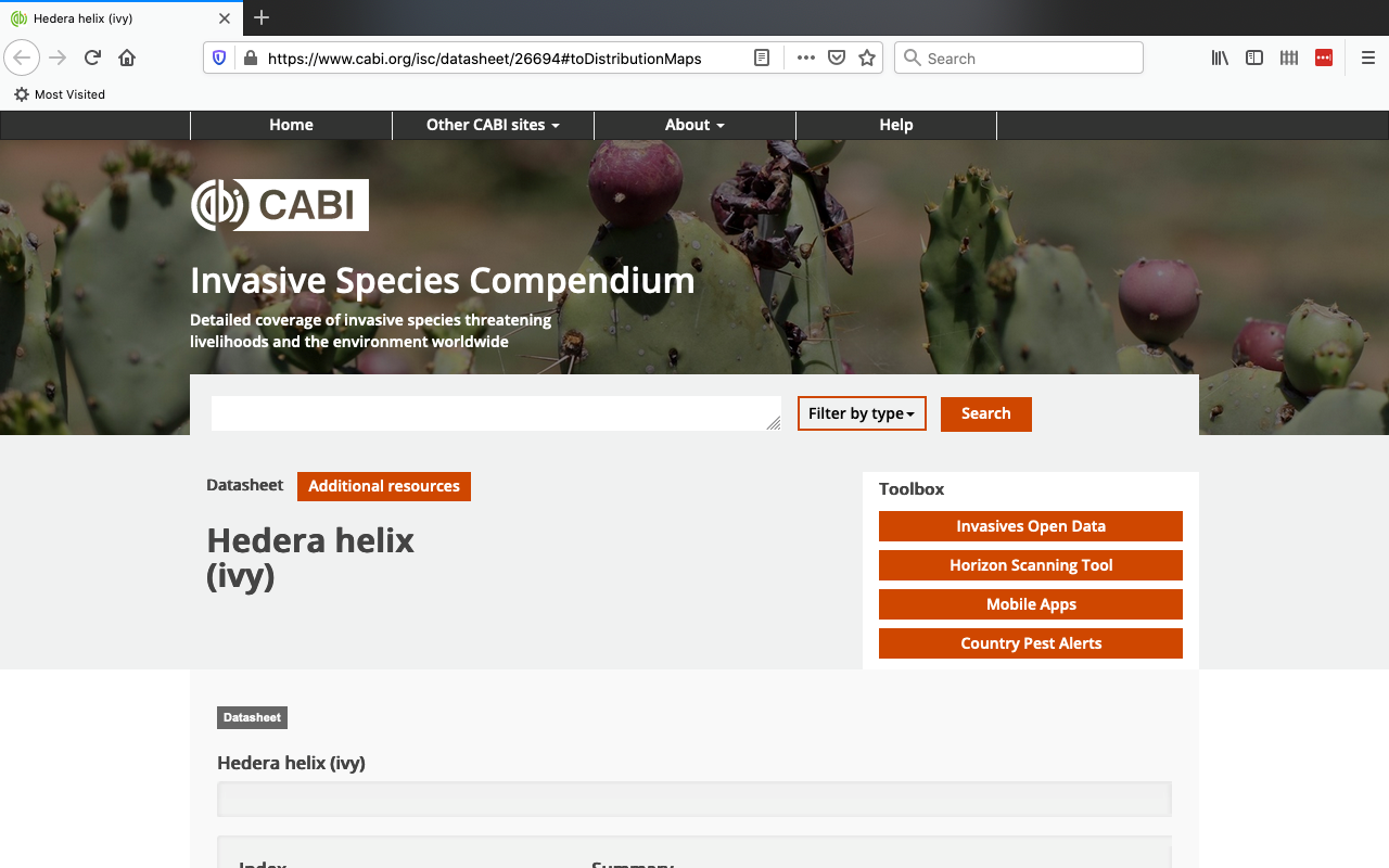
Figure 1: screenshot of the top of CAB International web page for English ivy (Hedera helix)

 

The major dataset obtained from that website was taken from a detailed “Distribution Table,” which contained geographical data about the presence or absence of English ivy in countries around the world (CAB International, 2020).

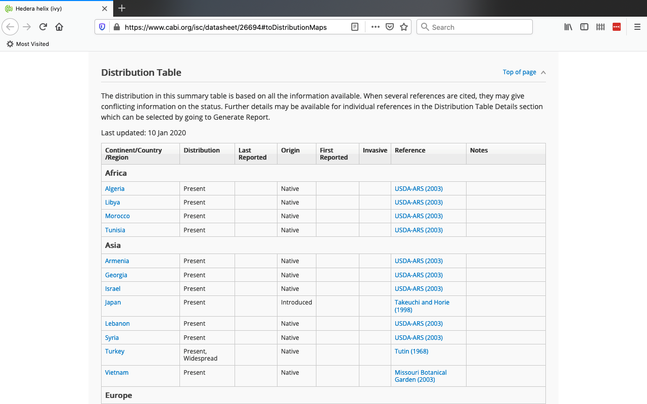
Figure 2: screenshot from CABI webpage showing the “Distribution Table” used for one of our large datasets

 

The dataset was downloaded as a CSV file from the full dataset that was used to make the above table and was copied into Google Sheets.

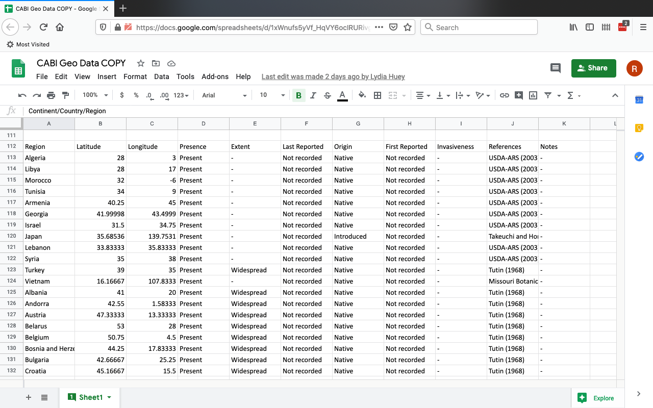
Figure 3: screenshot of the top of the original CABI dataset copied into Sheets

 

Two minor (smaller) datasets were taken from a table “Impact Summary” and an indented list “Risk and Impact Factors” (CAB International, 2020).

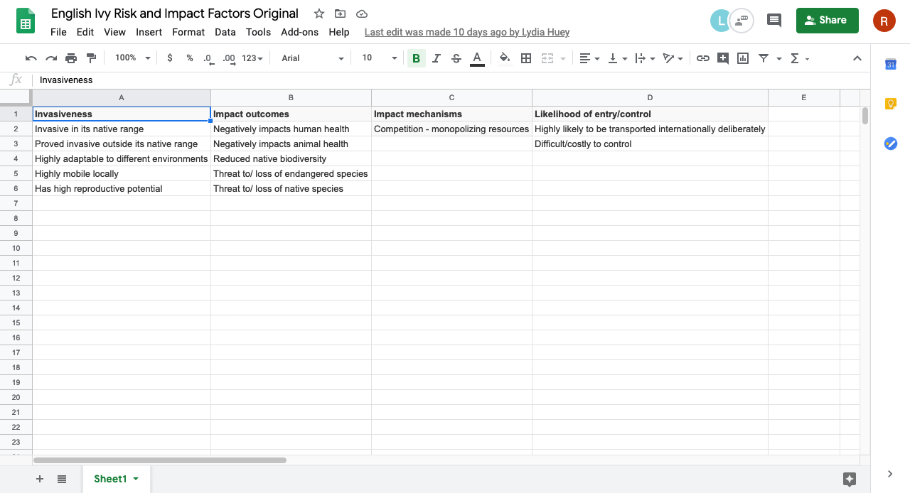
Figure 4: screenshot of the entire Risk and Impact Factors dataset copied into Google Sheets, converted into tabular format

 

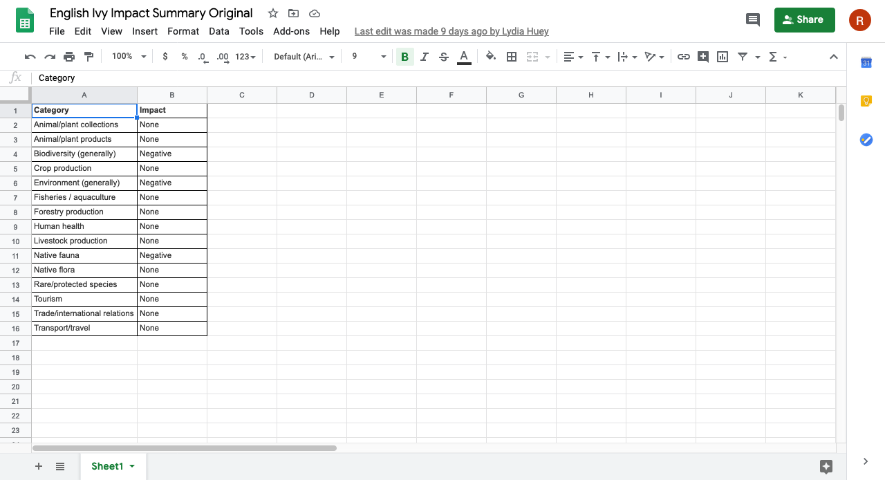
Figure 5: screenshot of the entire Impact Summaries dataset copied into Sheets

 

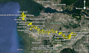
Another major dataset was extracted from E-Flora BC: Electronic Atlas of the Flora of British Columbia, using a polygon tool to select marks on a map that were located within British Columbia (E-Flora BC Distribution Map of Hedera helix (English ivy), 2020). The dot marks represented specific instances of a collector observing the presence of English ivy in that geographical location.

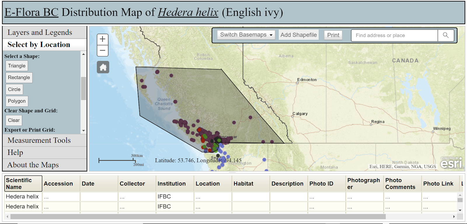
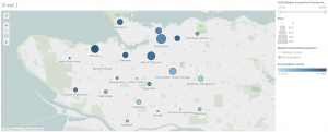
Figure 6: screenshot showing a recreation of the method used to obtain the data for occurrences of English ivy in BC

 

The dataset was downloaded as a CSV file and copied into Google Sheets.

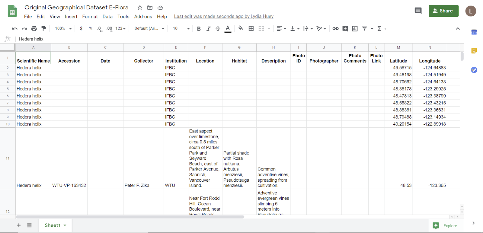
Figure 7: screenshot of the top of the original E-Flora dataset, showing the names of all the attributes in the first row

 

All datasets were taken from websites that included summaries of multiple scientific sources such as journal articles. 

Limitations of the Datasets:

While we felt that the CABI geographical data set came from a reliable source and was therefore trustworthy, we found that it did have limitations that made the visualization process challenging; the main limitation was the prevalence of fields with ‘null’ values. For example, “Invasiveness” was only identified as an attribute of English ivy in a few countries and provinces, and we did not know if its absence for any given item meant that the item was not considered invasive, or if the data was just not available. The dataset also included three former countries that were not recognized on the map in Tableau: Czechoslovakia, Federal Republic of Yugoslavia, and Serbia and Montenegro. Since our focus was mainly on BC, and since we were unsure if the borders of these countries would be consistent with existing borders as shown in Tableau, we decided to leave these three countries out of the final visualization; we recognize that this is may have skewed the data, but we hoped that our general global view and our more detailed view of English ivy in BC would not be greatly affected by this missing data. 

The E-Flora dataset had several limitations. To select the marks that occurred in BC, Lydia had to approximate using a polygon selection tool and then add in another row manually to include a mark that had not been included in the initial selection. Furthermore, when the CSV was downloaded, all the entered dates were garbled and had to be re-entered by manually locating each mark and typing in the correct date. Unfortunately, not all the data marks had corresponding longitudes and latitudes so those longitude and latitude for those marks had to be determined manually. These estimates were only somewhat accurate, so Lydia had to re-estimate many of the longitudes and latitudes using the information provided in the Location attribute column and Google map locations and determine estimated longitudes and latitudes from Google Maps. Since the original dataset had a high number of data points, due to time constraints, Lydia did not include two of the data sources within the dataset for occurrences of English ivy in BC. The E-Flora dataset only includes a small amount of data and Lydia suspects that the data was not collected evenly across BC. The localization of data in the Southwest of BC could be data could be due to both collection of data focused in that area and also the fact that English ivy may not be able to survive in less temperate areas of BC such as the Interior. For example, the CABI website states that  “[i]n North America (Midwest and New England states) it is reported that severe winter cold inhibits its spread (Moriarty, 2001) and in late autumn, flowers are susceptible to frost (Grime et al., 1988)” (CAB International, 2020).

Tools Used:

We used Microsoft Excel, Google Sheets, and Tableau Prep for data cleaning and wrangling. We used Tableau Desktop and Tableau Online to create our data visualizations. We used our chosen tools because we are somewhat familiar with them (for example, we learned about using the Tableau programs through class). We chose Google Sheets and Tableau Online to make it easier to work on the same file, including the option to work on the same file synchronously when needed. We used Canva (https://www.canva.com/) to create infographics to import into our Story, because it was free, it was recommended in class, and it allowed us to create image files such as PDFs, PNGs, and JPGs, which were easy to import into a Tableau Dashboard to be incorporated into the Story. 

Google Sheets and Microsoft Excel were more simple, more intuitive, and easier to use than Tableau Prep, especially since we are more familiar with them. Lydia found that Microsoft Excel was easier to use than Google Sheets since she has used Excel for a longer period of time and more often than Sheets. 

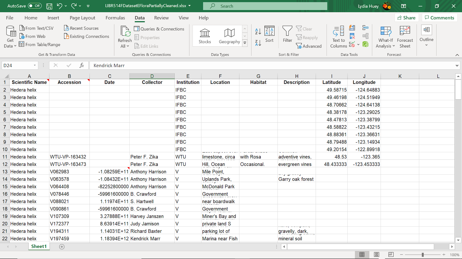
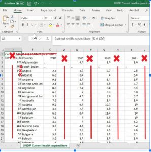
Figure 8: screenshot of using Excel to clean data; the dates were not properly formatted when the data was downloaded as a CSV, so Lydia was required to manually click on each dot mark on the E-Flora map and manually type in the correct date for each row.

 

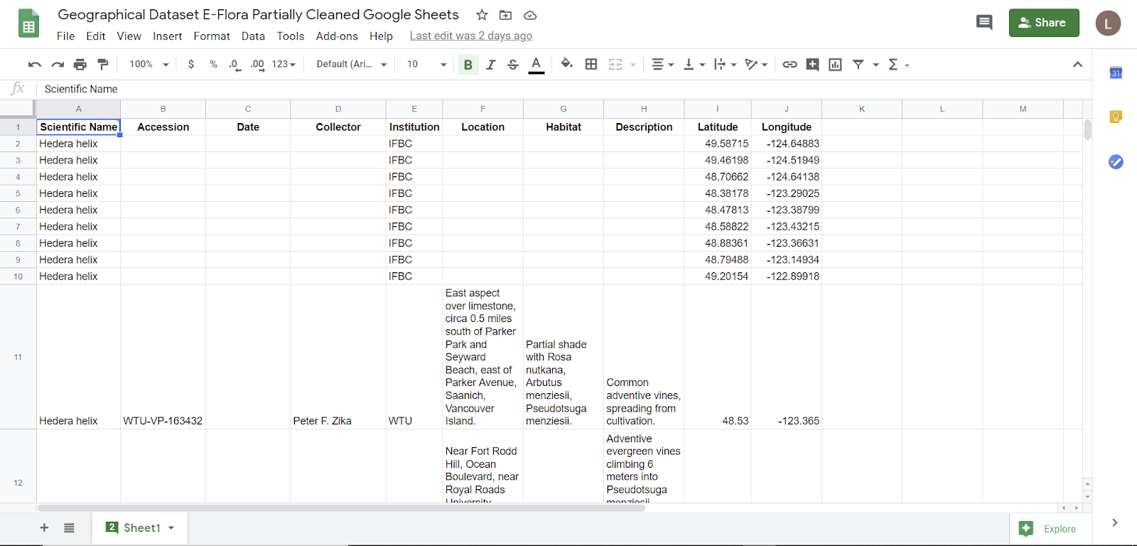
Figure 9: screenshot of using Sheets to clean data

 

Lydia found that Excel and Sheets had about the same functionality, including the useful function of the function “find and replace”. Although Tableau Prep was slightly harder to use since Lydia was less familiar with it, it was much easier to locate items with the same words within them and simply type to edit those items as a group. Tableau Prep’s use of aggregation and visualization of the data attributes made the data easier to survey as a whole and locate desired items, along with finding data that required editing. For example, one collector’s name was written in two formats and it was easy to group and replace those names in Tableau Prep. If one was using Excel or Sheets, the process would be more onerous.

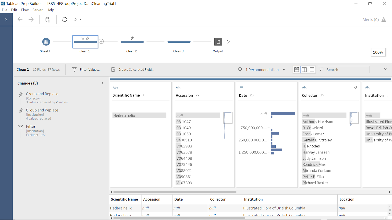
Figure 10: screenshot of Clean 1 in Tableau Prep showing cleaning steps

 

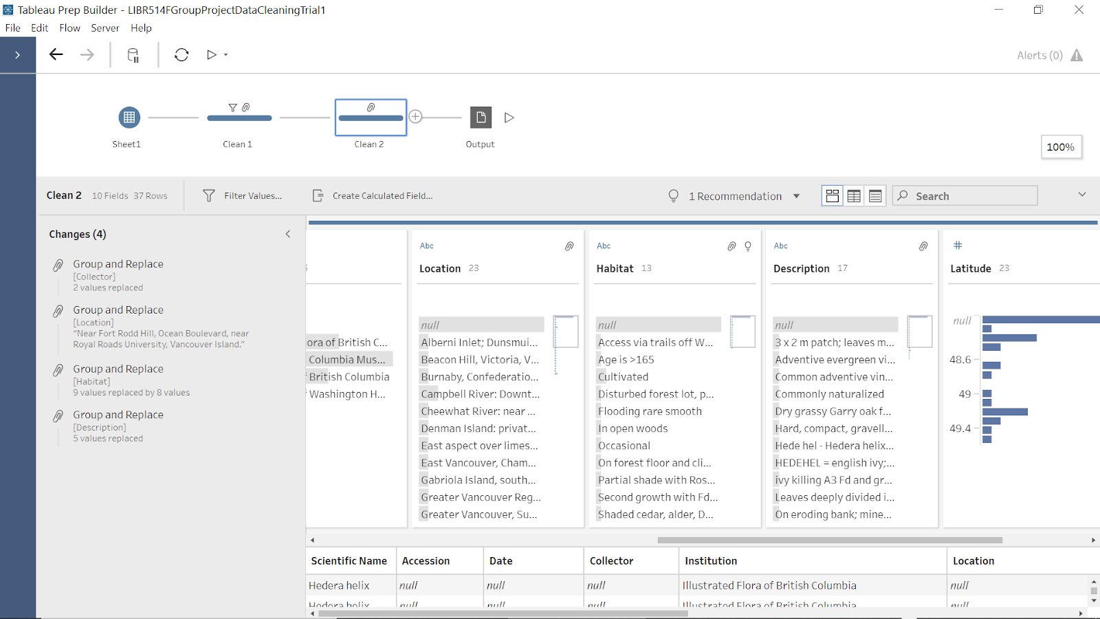
Figure 11: screenshot of Clean 2 in Tableau Prep showing cleaning steps

 

Tableau Desktop and Tableau Online were relatively straightforward to use to create information visualizations. Strengths include the “Show Me” function which can be used to quickly experiment with different visualizations and the Marks section, which allows for the data to be visually encoded using different visual channels such as size and colour. 

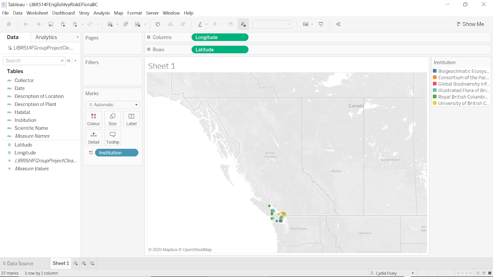
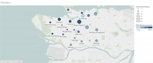
Figure 12: screenshot of a trial of visualizing the E-Flora dataset in Tableau Desktop

 

Another strength is that the Dashboard function allows importing text and images, along with visualizations created in Tableau, and the story function is useful for creating a narrative. One weakness of the Dashboard is that one can not easily move and align components within it: one has to use vertical and horizontal layout containers.

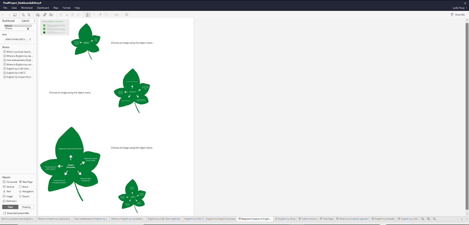
Figure 13: screenshot of Tableau Online showing a non-ideal layout of components (the four images with leaves are supposed to be readable and all the same size)

 

Two weaknesses are that the difference between “Tooltip” and “Detail” in the Mark section is not obvious, and that only a small number of map backgrounds are available in Tableau itself. One weakness of Canva (https://www.canva.com/) was that we could not change the size of the page with the free version to crop to an image so that it would fill the whole page.

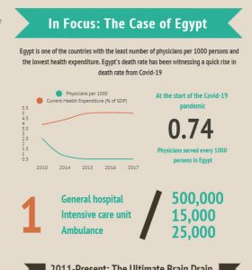
Figure 14: screenshot showing multiple pages of one of the small datasets made into an infographic in Canva

 

Design Process Analytic Steps:

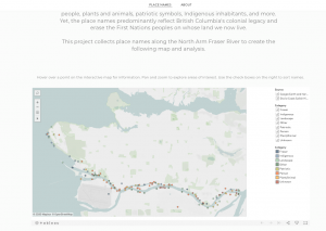
We knew the argument/idea to be communicated from the beginning and focused on presenting the data/evidence to communicate it through information visualizations. Since we knew the argument, we did not need to explore data visually to find patterns to make into visualizations. Since we are presenting to children aged 9 to 12 years of age, we had the idea of presenting the data in Tableau Story because it would be similar to a story with many pages in a book. We also decided to use infographics within our story to also make it visually engaging and simple for the children to understand. Additionally, since the audience is children, we tried to make our geographical visualizations simple to understand and analyze. For instance, we included four similar world maps emphasizing different attributes of the data, so that children could easily compare them visually. We also included opportunities for simple interactions such as hovering, highlighting, and filtering. 

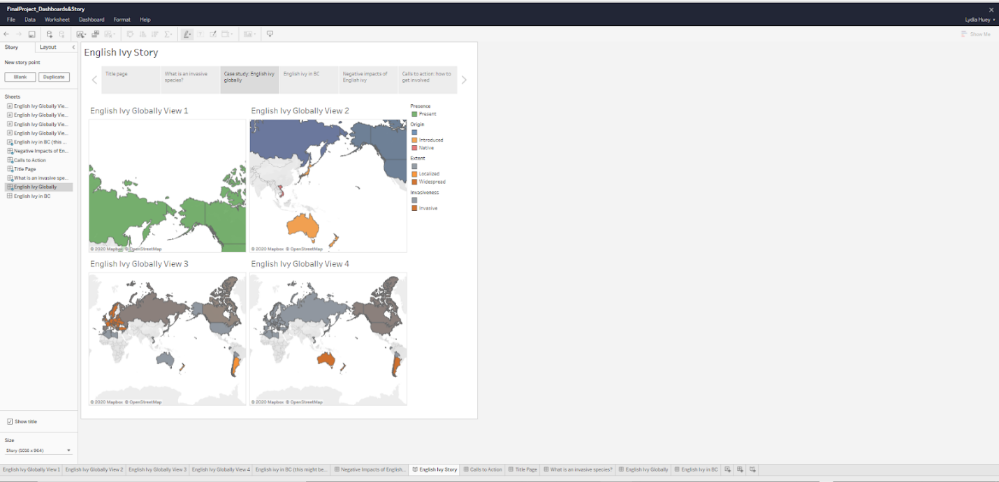
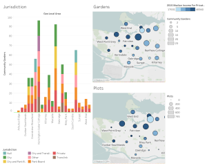
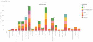
Figure 15: screenshot of a Tableau Story interactive dashboard draft in Tableau Online

 

We used the geographical information visualizations that the two source websites presented as inspirations for our own geographical information visualizations. 

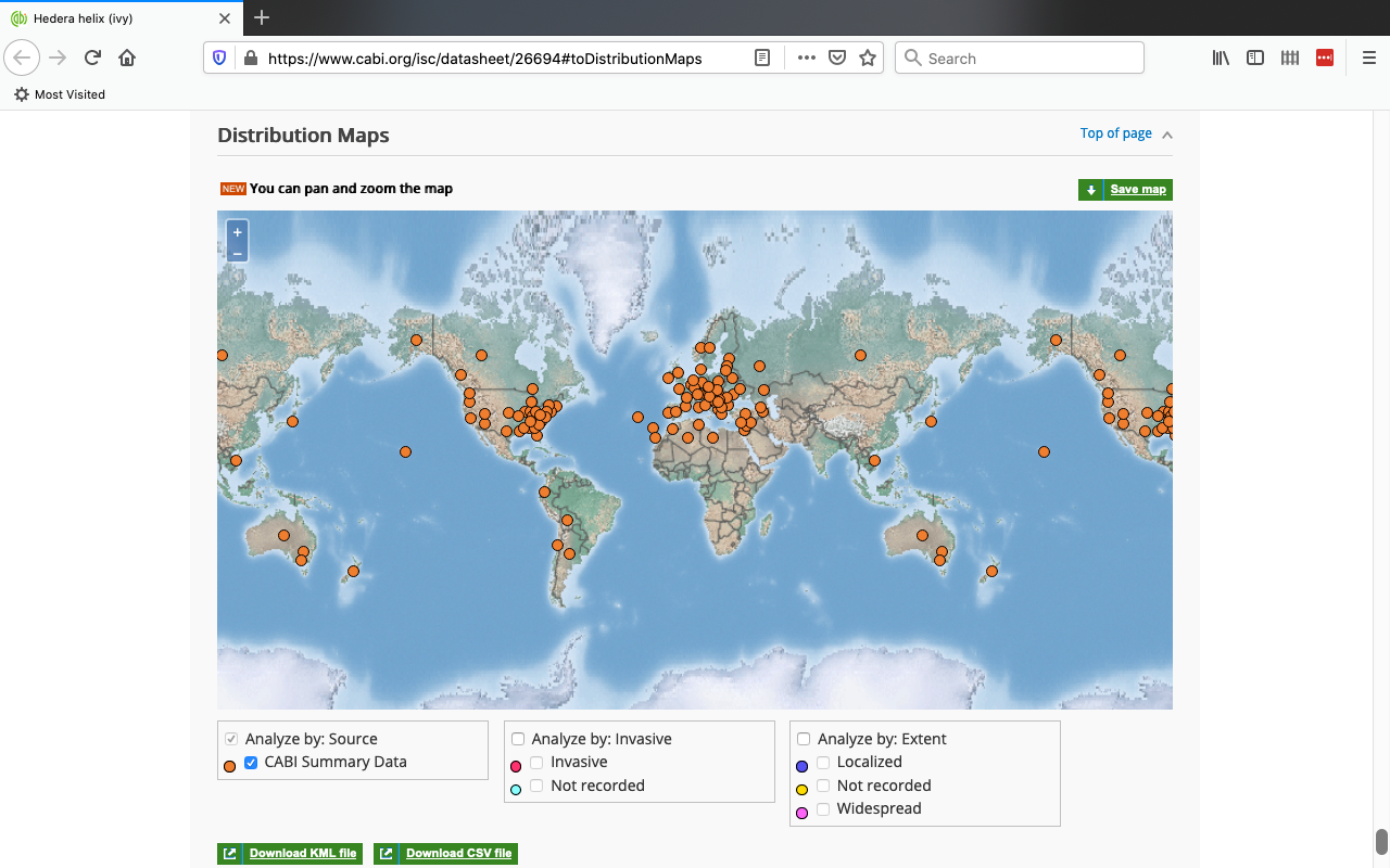
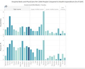
Figure 16: screenshot of an information visualization created by CABI

 

Design Process and Principles: 

We decided early in the process of analyzing our data sources that geographical maps would be our main idiom. This was partly because of the nature of the data, and partly because we felt that maps would be an intuitive form of visualization for children still learning how to understand visualized data. Munzner (2015) explains, if “the given spatial position is the attribute of primary importance because the central tasks revolve around understanding spatial relationships…the right visual encoding choice is to use the provided spatial position as the substrate for the visual layout”  (pp. 179-180). To meet the requirements of expressiveness, we used mostly identity channels because we were working with location-based and categorical data rather than quantitative data (Munzner, p. 99). To meet the requirements of effectiveness, we considered channel rankings as described by Munzner (2015): we used spatial region and color hue because these are the most effective channels for categorical data (p. 101). Our choice of geographical maps as an idiom also followed the effectiveness principle because, as Munzner states, “the most effective channel of spatial position is used to show the most important aspect of the data” (Munzner, 2015. p. 180). 

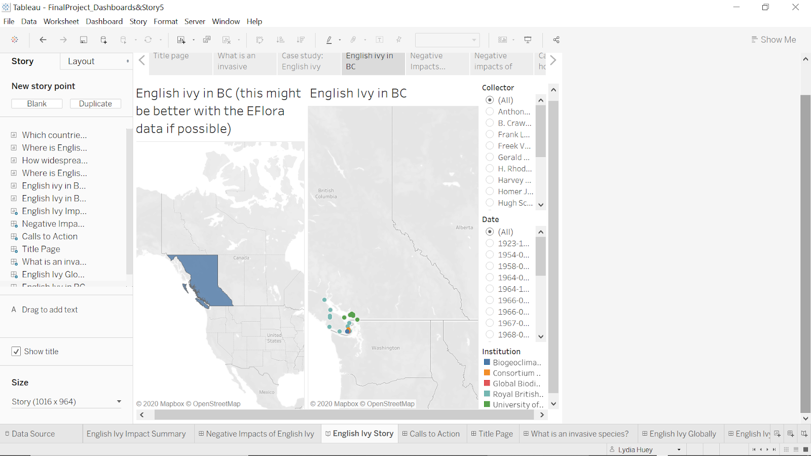
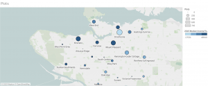
Figure 17: screenshot of a trial of creating an interactive geographical dashboard in Tableau Desktop

 

We attempted to follow the principle of separability by using separable or mostly separable channels when we were trying to indicate “two different data attributes, either of which can be attended to selectively” (Munzner, p. 108); for instance, the two main channels we used were the separable channels of position and colour hue (p. 108), to show the locations of English ivy at the same time as other attributes such as “Invasiveness.” Following the principle of discriminability was not one of our main challenges (Munzner, p. 106); because much of our data had attributes that only included a small number of categories (for instance, “Present” or “Null”), we did not need to consider whether our selected channels allowed for large numbers of bins. We also attempted to create visual popout using hue and saturation, and tried to limit distractors (Munzner, pp. 109-110). The following images show how we adjusted the default colours in a view to increase visual popout using both hue and saturation.

Figure 18: screenshot of Impact Summary initial colours

 

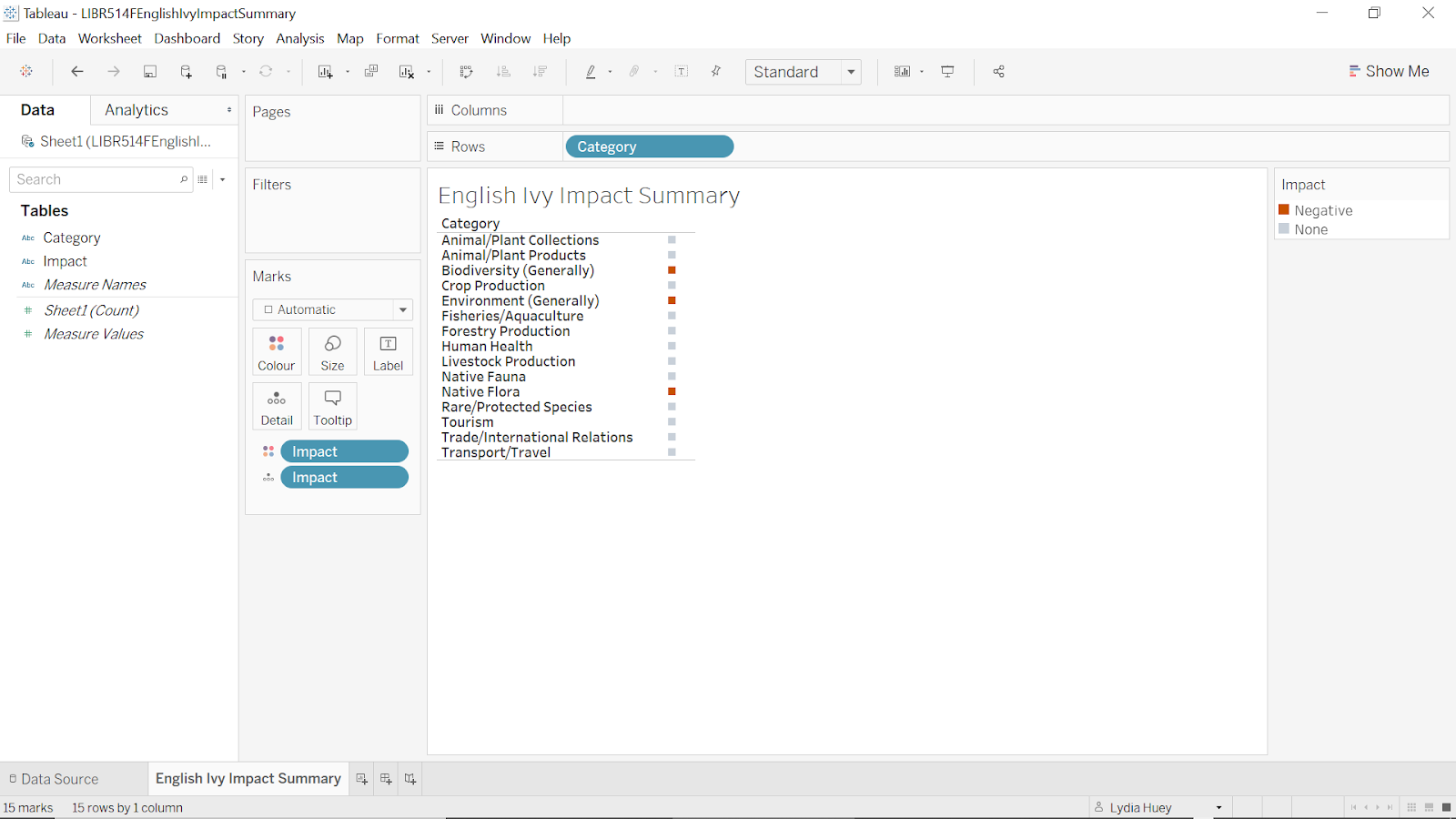
Figure 19: screenshot of Impact Summary final colours

 

Using Canva, we created infographics to present qualitative data such as definitions of concepts and terms. We aimed to follow Lankow, Crooks, and Ritchie’s (2012) principles of utility, soundness, and beauty. Because we chose a narrative form of communication rather than an explorative one, we were able to meet the principle of utility by leading our viewers “through a specific set of information that tells a predetermined story”; we also tried to follow Lankow et al.’s recommendation for narrative communication, to “focus on audience appeal and information retention” (p. 199), by combining visuals with text and attempting to engage readers’ interest with questions. We attempted to follow Lankow et al.’s principle of soundness, by choosing a topic that we felt would be interesting and relevant to at least some viewers in our chosen age group; we feel that the data we chose is trustworthy, and we endeavoured to present it with integrity (p. 200); however, we did face limitations which we have discussed in our description of the data. We also strove to meet Lankow et al.’s requirement of beauty, ensuring that the aesthetic style of our infographics was consistent with the story we wanted to tell and was appropriate for our audience (p. 201). We decided to use some illustration in our infographics (including both images available on Canva and photographs found elsewhere), because we felt that they would make the topic more interesting and engaging, and because certain concepts, such as the negative impacts of English ivy, seemed easier to understand if shown in visual form (Lankow et al., p. 204). 

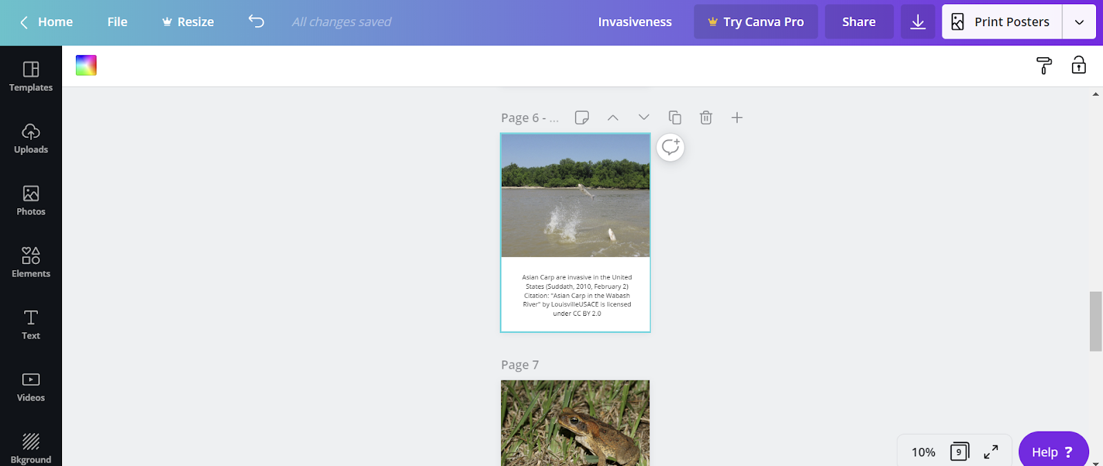
Figure 20: screenshot showing images and text being combined in Canva

 

In this way, we tried to incorporate what Lankow et al. call “audience appropriateness” and “content appropriateness” into our design (p. 206). Lankow et al. note that because a narrative infographic has a pre-established message, illustration is often more appropriate than it would be in an explorative infographic (p. 205).

Story Description:

Our story is about invasive species: introducing what they are to children aged 9 to 12, presenting a case study of an invasive species, communicating that invasive species have a negative impact on the world, and having a call to action. We also wanted to introduce information visualizations and how to use them. Our story moves from general to specific (invasive species to English ivy), and communicates ideas of how children can get involved to decrease the negative impact of invasive species. This story is credible because it is based on scientific evidence of negative impacts of invasive species. It is relevant because those negative impacts can be quite severe, impacting humanity and other organisms as a whole.

Pros and Cons of Designs:

One benefit of our design is that the story format clearly separates each topic into its own story point, so that viewers can concentrate on one story point at a time and so that we can guide them through the narrative. One drawback of this design may be that viewers who want to engage in more active analysis may have difficulty comparing information across different pages. The use of infographics allows readers to understand ideas through a combination of text and images; we hope that this combination, common in children’s educational materials, will allow viewers to combine their visual and textual literacy skills to help them understand and interpret the data. One limitation in Tableau’s map feature is that it is distorted to make the northern hemisphere seem larger than the southern hemisphere. While two-dimensional world maps are necessarily distorted, we worried that the relatively large size of the northern hemisphere could distort a viewer’s understanding of the prevalence and locations of English ivy globally. 

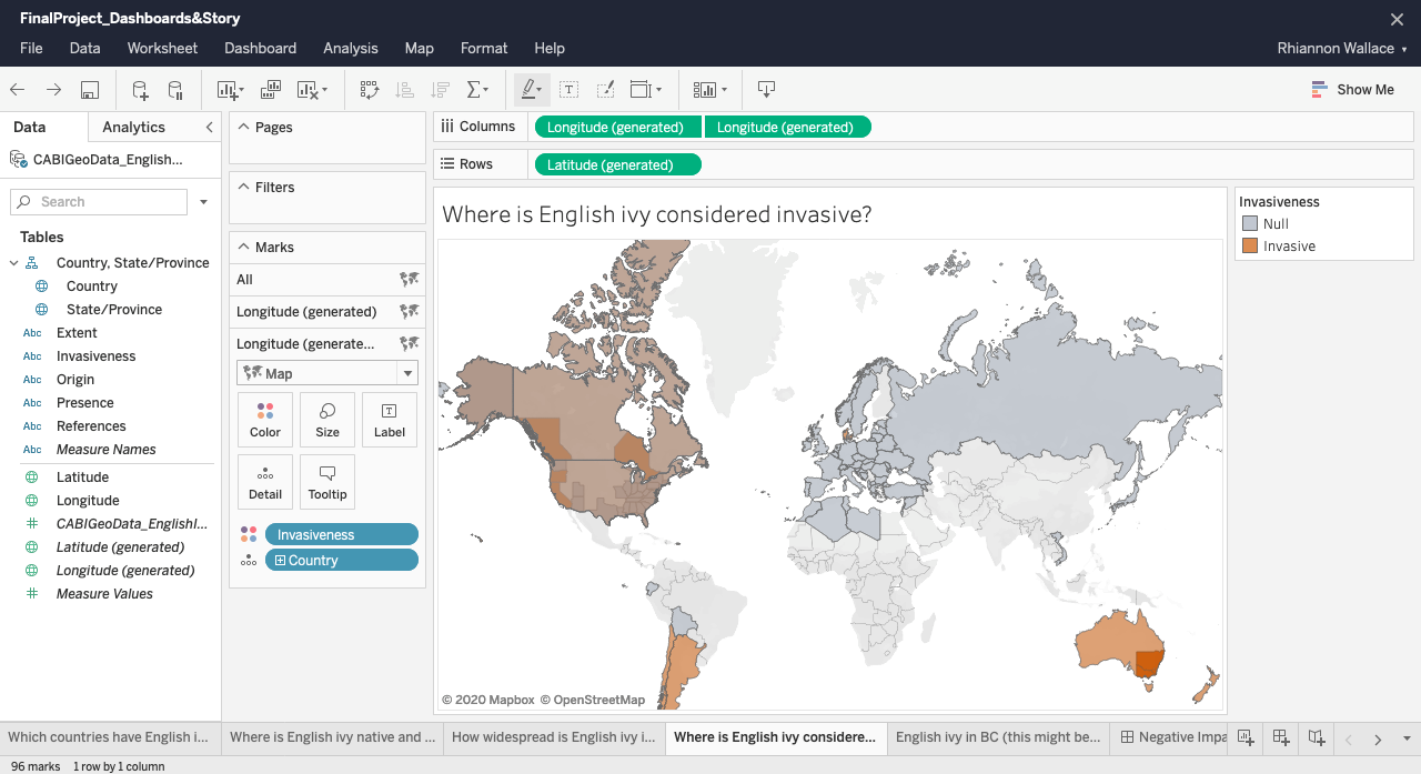
Figure 21: screenshot of a map in Tableau Online with distorted sizes of geographical land masses

 

This was less problematic in our more focused map of BC. Another design challenge related to the map idiom was being able to show presence or absence of English ivy in different countries, without misleading viewers to associate the area of the country with the amount of ivy; for instance, Canada or Russia does not necessarily have more English ivy than a smaller country like the UK. If we had been able to find a dataset pinpointing the exact regions where English ivy can be found in each country, we would have been able to create a more accurate view. Another limitation was that we were unable to find a way to incorporate audio narration into our Tableau Story. While we worried that this may make the story more difficult for some students to follow, we imagine that a teacher could guide students through the resource in a classroom setting.

References:

CAB International. (2020). Hedera helix (ivy) [Online datasheet]. Retrieved from 

        https://www.cabi.org/isc/datasheet/26694

E-Flora BC. (2020). E-Flora BC distribution map of Hedera helix (English ivy) [Interactive 

        map]. Retrieved from https://linnet.geog.ubc.ca/eflora_maps/index.html?sciname= 

        Hedera%20helix&BCStatus=Not%20listed%20provincially&synonyms=%27 

        Hedera%20helix%20var.%20hibernica%27&commonname=English%20ivy&PhotoID 

        =14929&mapservice=VascularWMS

Lankow, J., Crooks, R., & Ritchie, J. (2012). Infographics: The power of visual storytelling. 

        Retrieved from https://ebookcentral.proquest.com/lib/ubc/detail.action?docID=882721

Munzner, T. (2015). Visualization analysis and design. doi:10.1201/b17511

Province of British Columbia. (2020a). Applied design, skills, and technologies 5 [Web page]. 

        Retrieved from https://curriculum.gov.bc.ca/curriculum/adst/5/core

Province of British Columbia. (2020b). Science 5 [Web page]. Retrieved from 

        https://curriculum.gov.bc.ca/curriculum/science/5/core

Suddath, C. (2010, February 2). Top 10 invasive species. Time. Retrieved from https://time.com/

Ursyn, A. (2016). Chapter 1: Teaching and learning science as a visual experience. In A. Ursyn 

        (Ed.), Knowledge visualization and visual literacy in science education (pp. 1-27).      

        doi:10.4018/978-1-5225-0480-1.ch001

Zheng, R., & Wang, Y. (2016). Chapter 11: Optimizing students’ information processing in 

        science learning: A knowledge visualization approach. In A. Ursyn (Ed.), Knowledge 

        visualization and visual literacy in science education (pp. 307-329). doi:      

        10.4018/978-1-5225-0480-1.ch001

by Janet Hilts & Eleanor Ren 

Link to our final project can be found here

Recently, the topic of equity, diversity and inclusion has been back in the spotlight. As information students and women in the workforce, our information visualization project focuses on the topic of equal work and analyses gender differences in job positions and earnings. 

The British Columbia Human Rights Code prohibits discrimination in hiring and requires equal pay regardless of gender identity and expression (Government of British Columbia, 1996). However, we believe that equal pay for the same kind of work does not mean the equality of work. Even in the progressive city of Vancouver, there is still an existing unbalanced hiring pattern where women are in a disadvantageous position. 

During the initial research, we found a dataset from the City of Vancouver Open Data Portal titled Workforce pay rates and gender. The dataset is current, with data from 2019. Because we are accessing this dataset through the municipal government’s repository, we also believe this data is credible, and are not aware of biases in it.  

Meanwhile, we found an article from Vancouver Sun, which noted that three-quarters of the women who work in BC’s public sector are in the lowest salary bracket, while men are massively overrepresented in the higher pay scales (Culbert & Griffiths, 2020). Based on this evidence, we believe that the dataset we chose is meaningful and worth studying. Thus, we elaborated our topic to be the current gender wage gap situation in Vancouver’s public sector, with a focus on gender distribution within different positions. 

Overall, our project intends to communicate knowledge about the pay gap between genders among City of Vancouver employees.   With the main goal of raising people’s awareness among Vancouverites while calling on the City of Vancouver to make equal choices during the recruitment process, our target audience will be the general public.

The Dataset

The original dataset has 189 items (rows) and 8 attributes (columns). The attributes include categorical and quantitative data types, including “Year”, “Classification”, “Exempt/Union”, “Minimum hourly rate”, “Maximum hourly rate”, “Women”, “Men”, and total. The dataset was compiled internally by the Human Resources – Equity, Diversity and Inclusion Office (City of Vancouver, 2020). It is well structured and does not appear to include inconsistent data formats, duplications, or errors.

To clean the data, we removed the irrelevant column “Year” and deleted the summation record “Total”. To make sure the consistency and informativeness of the variables, we renamed some attributes to be more descriptive as well. 

Since there are 187 different classifications within the dataset, readers from the general public may find detecting hiring patterns challenging. Thus, we emailed the dataset publisher and got a spreadsheet from a City official that has job titles for each classification (see attachment). Based on job duties, we added an attribute named “Classification Group”, and sorted all the jobs into 31 categories, for example, Admin Management, Trades, and so on. Additionally, to examine the influence of unions in equal pay, we added another attribute called “Unionized”, and assigned all entities a “Yes” or “No” value.

The Tools

In general, we used five tools to create the visualization, the infographic, and the final webpage: Excel, Canva, Wix, Tableau Desktop, and Adobe Color Wheel.

First, we used Excel to process the data and edit the idioms. Because our data does not need sophisticated cleaning, we used the software that our team members are the most familiar with rather than Tableau Prep to clean it. Meanwhile, when creating the infographic, the average salary and the total number of men and women need to be calculated. By using the formulas function and the AutoFill feature, all these tasks can be easily achieved.

Second, we used Canva as the primary tool to create the infographic. As an all-in-one online graphic design platform, Canva is easy to use and share design as a group, which is super helpful in the quarantine period. Although we were using the free version, it still has enough resources for us to design and make the infographic. One weakness of Canva is the inability to customize the chart colour, even for prime members. Thus, we had to change the colours of the pie chart on Excel and paste the copied idiom to the platform. Also, Canva can’t do some fine/advanced design. We can’t adjust the length of the template and delete the unnecessary parts. Designers can’t adjust the sizes of the elements in a precise way – we can only zoom in and out with the mouse/control pad.

For the final deliverable, we chose to display our visualizations and story on a simple webpage, so we used Wix since it is free, simple to use, and allows Tableau visualizations to be embedded. We also used Adobe Colour Wheel to choose colour combinations that are aesthetically pleasing and impactful for our webpage and infographic. 

Last, we used Tableau Desktop, the tool that we have received training in during class to make the visualization. The software is powerful, especially with the calculated field function allowing further manipulation of the data. It also helps us to add the interactive feature of the website without knowing much JavaScript knowledge. However, Tableau is the tool that requires the most professional training and is the most expensive. The other thing we found in Tableau is that it has no function to calculate the weighted average. Thus, we have to “cheat” Tableau and create a vertical line ourselves to present the “real average” of our dataset.

Initial Analyses

During the design period, our team organized two Zoom conferences, where we set three directions for data research: the overall distribution of male and female in the City of Vancouver jobs, the percentage of male and female in high-income positions, and whether the labour unions contribute to equality.

To find patterns within these three directions, our team members played around with the data with the help of Tableau Desktop and Excel and found there was an unbalanced position distribution between men and women. Therefore, we further focused on presenting the evidence, and went ahead and tried a variety of Tableau idioms. In the end, we decide to present the data in two ways: an overview infographic and interactive visualizations (the bar chart and scatter plots).

Design Process

To comply with the principles of effectiveness and expressiveness, we first chose the spatial region channel and put classification groups on the horizontal position on the common scale to convey the identity attribute in the first visualization (Fig. 3). Then, we use the most effective magnitude channel, position, to present the proportion of women in different groups (numeric attribute).

The advantage of this design is its simplicity. Audiences can easily tell the percentage of women in each job classification group by the location of the dots. However, this also sacrifices the representation of the group of another statistic: the specific numbers of men and women in each group. Since the purpose of our design is to provide the big picture, audiences interested in more detailed information can access the clean data we provided in the attachment and produce with their own tools.

In our second visualization (Visualization 3-2), we chose to represent the data using a stacked bar chart to show the relative proportions of parts of a whole, in our story, the number of women vs the number of men able to earn maximum hourly wages, from lower to higher wages. Munzner (2014, pp 151-53) indicates a stacked bar chart is the proper idiom to express 2 categorial key attributes – men and women – and 1 quantitative key attribute – max hourly rate. 

The primary pro of this visualization is our choice of idiom, which is able to express the story of women being over-represented in lower-paying positions and less represented as pay increases, vis-a-vis men. Helping to make this aspect of our story clear, we chose the second-best identity channel to express categorical attributes, colour hue, to express the categorical attributes of men and women, while the magnitude channel position-on-a-common-scale expresses the number of employees. 

A weakness of stacked bar charts, especially one with a wide range of values on the y-axis, is comparing the length of the stacked components can be challenging (Munzner, 2014,  pp. 151-52). As a result, this chart may over-complicate the details in the story we want to tell. We feel that judging the heights of the stacked components is somewhat tricky when viewing all pay rates, but using the filter helps to see differences better. 

Also following Munzner’s guidance on idioms (2014, pp. 146-148), for our third visualization (see Fig. 6), we used a scatterplot to encode two qualitative value variables (max hourly rate and number of women employees) in the spatial channel while adding a categorical attribute (Union Yes/No) encoded with the colour (hue) channel. Munzner explains this idiom is useful for seeing correlations, and we hoped with it, we could tell the story that Unions are part of the gender wage gap problem. With this visualization, we hoped readers could see correlations between wage and number of employees while comparing how this correlation is or isn’t affected by unionization, and between unions as well.

In the fourth visualization (see Fig. 5) we also encoded the number of men employees to allow for comparison between the distribution of men and women employees. These visualizations are effective in helping us to tell our readers that there are differences between unions and between union vs non-union positions concerning the distribution of women over the pay scale. However, their main pro is they tell the story that unions are not mitigating the gender wage gap. 

A major con of this idiom for telling this story, though, is the scatterplot is not intuitive to many people. As a result, members of our user group may not be able to derive much meaning from this visualization. Another weakness is that many users may have trouble comparing the men and women distributions since they may not understand the trend lines we added. (We hoped the lines angling downwards in the women’s chart would help to tell the story that as wages increase in both unionized and -non-unionized positions, fewer and fewer women employees are represented).

Infographic is the first presented and the most important part of our storytelling. To ensure the consistency and consistency of all the content, we first decided on the theme colors of the website: blue (#087CB4) and brown(#B56807). The choice of blue we made referred to the same colour used by the City of Vancouver and the Open Data Portal website, and we used this colour to present men, the “majority”. Then, we correspondingly chose its complementary colour, brown, to present women in our infographic.

Following the principles of utility, soundness and beauty, we replaced the default font Knewave with Montserrat Extra, which is more formal and easier to read. Also, we strictly limited the number of words in our infographic and emphasized the comparisons by using idioms and the diagram. 

That said, a merit of our infographic is it is “[c]ommunicating a message worth telling [and so] provides readers with something of value” (Lankow et al., 2012, p. 200), which should entice many readers to keep reading to find out more about the women workers’ situation. As well, we chose intuitive and easy-to-comprehend idioms for our charts: a bar chart and pie chart.  Lankow et al (2012) explain that using bar charts is highly valuable in helping the reader understand what is going on and pie charts, despite their criticism, are useful for “…communicating big ideas quickly” (Lankow et al., 2012, pp. 213, 216). With these simple charts, we quickly introduce the story of how women workers are faring in a way that a large number of our readers can easily grasp.

Accordingly, a weakness of our infographic is it may emphasize comprehension too much and appeal too little. Our goal was to make a clear and intuitive narrative infographic to “… leave readers with a specific message to take away” (Lankow et al., 2012, p. 199), that women workers at the City of Vancouver are fewer and earning less than men. But because our design is quite simplistic and safe, we may not catch viewers’ attention sufficiently enough to compel all readers to read the rest of our story.

Our Story: the Website

In the final deliverable, the news-like webpage we created, we concluded the true but disappointing reality: despite Vancouver’s image as a progressive city, its municipal government’s workforce has not escaped the gender wage gap. Taken together, we combined text, an infographic and visualizations to help to tell the story of this wage gap and give readers the opportunities to uncover trends that reveal why women are not earning as much as men at the City of Vancouver. 

First, our infographic provides an overview of how women employees are faring, answering the questions “How balanced is the workforce’s gender representation?”, “How much are women able to earn per hour on average compared with men?” and last, “Are an equal number of women earning the biggest bucks yet?.”  Answering these questions, our infographic provides a snapshot that, yes, a gender wage gap exists at the City of Vancouver. 

Our visualizations fill out our story, adding complexity and details, offering insight into how this wage inequality persists. One visualization helps to show that women workers are overrepresented in classifications of work dominated by jobs “traditionally held by women,” such as administration, instruction, and service and support roles. We make the connection to the gender wage gap that these jobs tend not to be as high paying as more masculine jobs, including skilled trades such as mechanics, machinists, and so on.

Our visualizations also help to reveal the sticky floor and glass ceiling that holds women back from earning as much as men (McInturff & Tulloch, 2014). We reveal the story of how women are not nearly as evenly distributed across the pay scale as men, with many women in positions toward the pay scale’s lower end. Last, since most City jobs are unionized, we examine what role the various unions play in our story.  We reveal that despite unions helping to mitigate the gender wage gap overall in Canada (McInturff & Tulloch, 2014), the women workers represented by unions at the City of Vancouver are not faring better than their non-unionized counterparts.  In short, we reveal that unions remain part of the gender wage gap problem.

References

City of Vancouver. (2020). Workforce pay rates and gender. City of Vancouver Open Data Portal. [Data set]. Retrieved June 1, 2020 from https://opendata.vancouver.ca/explore/dataset/workforce-pay-rates-and- gender/information/

Culbert, L., & Griffiths, N. (2020). Public sector salaries: Where are the women? In BC, not many are near the top of the pay scale. Vancouver Sun. Retrieved May 31, 2020 from https://vancouversun.com/news/local-news/public-sector-salaries-where-are-the- women-in-b-c-not-many-are-near-the-top-of-the-pay-scale

Government of British Columbia. (1996). Human Rights Code. Bclaws. Retrieved May 31, 2020, from http://www.bclaws.ca/civix/document/id/complete/statreg/00_96210_01. 

Lankow, J., Ritchie, J., & Crooks, R. (2012). Infographics: the power of visual storytelling. John Wiley & Sons, Inc. 

McInturff, K., & Tulloch, P. (2014). Narrowing the Gap: The difference that public sector wages make. Canadian Centre for Policy Alternatives. https://www-deslibris-ca.ezproxy.library.ubc.ca/ID/244703

Munzner, T. (2014). Visualization analysis and design. A K Peters/CRC Press. https://doi.org/10.1201/b17511

 

Continue reading →

Clara Gimenez-Delgado & Caroline Halley

Access our (almost) final version here

What’s the Story?

The last two decades of the 20th Century saw an exponential increase in Indigenous resurgence movements claiming the implementation and extension of what the government of Canada had called “Aboriginal Rights.” One of those concerned the right to fish and sell all traditionally harvested species within First Nations territories.

As a result of continuous litigations, in 1990 the Supreme Court of Canada ruled that Indigenous peoples fishing for food, social, and ceremonial purposes had priority over commercial fishing after demands of conservation had been met (Aboriginal Fisheries in British Columbia, Indigenous Foundations, UBC). A direct consequence of said ruling was the launch of the Aboriginal Fisheries Strategy (AFS) in 1992, with Fisheries and Oceans Canada (DFO) overviewing it. Several projects followed the creation of the AFS, and collaboration between DFO and different Nations started. However, the accords and agreements had to be reached individually, nation by nation, and case by case, making Reconciliation efforts slow and frustrating for the communities.

Continue reading →

References

Depression. (2020, January 3). World Health Organization. Retrieved May 31st 2020. https://www.who.int/news-room/fact-sheets/detail/depression
Feenstra, Robert C., Robert Inklaar and Marcel P. Timmer. Our World in Data. (2019). National GDP. [Dataset] https://ourworldindata.org/grapher/national-gdp
Kessler, R. (2011). The Cost of Depression. Psychiatric Clinics of North America, (35)1, 1-14. https://doi.org/10.1016/j.psc.2011.11.005
Koski, B. & Legg, T. J. (2020, June 3). Depression: Facts, Statistics, and You. Healthline. https://www.healthline.com/health/depression/facts-statistics-infographic#1
Ritchie, Hannah, and Max Roser. Our World in Data. (2018). Mental Health. [Dataset] ourworldindata.org/mental-health#depression.
Factors that Affect Medical Costs
References:

Abd El-Galil, T. (2019, Jul 29). Egypt’s Doctors are Fleeing, Leaving Behind a Physician Shortage. Al-Fanar Media. Retrieved from: https://www.al-fanarmedia.org/2019/07/egypts-doctors-are-fleeing-leaving-behind-a-physician-shortage/
Burn-Murdoch, J., et al. (2020, April 26). Global coronavirus death toll could be 60% higher than reported. The Financial Times. Retrieved from: https://www.ft.com/content/6bd88b7d-3386-4543-b2e9-0d5c6fac846c
Dale, B., Stylianou, N. (2020, June 18). Coronavirus: What is the true death toll of the pandemic? BBC News. Retrieved from: https://www.bbc.com/news/world-53073046
Egypt’s Medical Syndicate refuses suggestion to give pharmacists doctor’s license. (2020, May 5). Egypt Independent. Retrieved from https://egyptindependent.com/egypts-medical-syndicate-refuses-suggestion-to-give-pharmacists-medical-license/
Findlay, S. & Singh, J. (2020, June 11). Delhi accused of under-reporting coronavirus deaths. The Financial Times. Retrieved from: https://www.ft.com/content/5049c66f-449d-4a13-ba1c-f95893b60597
Global Health Workforce Statistics, OECD, supplemented by country data. World Health Organization.