
Lab 3 was about Geographically Weighted Regression, most especially, the lab focussed on the case study of children’s social skill scores in Vancouver, Canada. The first section of the report introduced what GWR is, and the second part focussed on evaluating the use of GWR in respect to the case study of explaining social skills score of children in Vancouver. The final part provided other examples of when GWR can be useful to use in order to explain spatial relationships.
What is GWR?
Geographically Weighted Regression (GWR) is a popular method used within the field of Geographic Information Science that explores spatial data analysis, and models spatial relationships.The foundational idea behind GWR is to explore the relationship between a dependent variable (Y), and a single or multiple independent variables (X), as it varies across the landscape.
Regression analysis enables one to “model, examine, and explore spatial relationships and can help explain the factors behind observed spatial patterns.” Such models can also be used to predict future patterns. The Ordinary Least Squares (OLS) regression is the most well-known technique. It calculates a global model for the variable you are trying to understand; only one equation is generated for the entire study area. However, another spatial regression technique which is increasingly being used is the Geographically weighted regression which provides a local model of the dependent variable to be explained – in such a technique a regression equation is calculated for every feature point in the data set – thus taking into accounts each feature’s closest neighbors.Unlike, Ordinary Least Squares Regression analysis the GWR analysis looks for geographical differences and looks at spatial variations in the relationship between the dependent variable and the independent variables.
The geographically weighted regression is an extension of the linear model which allows for its analysis/model to vary over space. From its output, it is, therefore, possible to find areas where the independent variables have a positive relationship with the dependent variable, whilst in other places, it may be negative.
By exploring spatial heterogeneity GWR addresses the geographical thinking assumption that spatial phenomenon varies across a landscape. The model is not looking at variation over the overall data space. Instead, it is used using a “weighted window” over the data, analyzing values and estimating coefficients at specific points by looking at the surrounding neighbors.Typical regression-based models, such as Ordinary Least Squares ignore that assumption and thus provides a less accurate explanation of spatially varying relationships. This is not to say that the OLS regression is not appropriate and accurate. Indeed, aspatial models can, in some cases, lead to a high correlation between the model and estimated values from the independent variables. Nevertheless, in most cases, and while analyzing geographically sensitive topics, the GWR model will increase the accuracy of the model and in general have a higher fitness between the model and reality. Consequently, geographically weighted regressions can be seen as an improvement over using regressions such as OLS. Ordinary least squares regressions model a global relationship whilst GWR use neighboring data values to estimate spatial relationships and thus computes more accurate predictions.
To provide a local model for the explanatory variables, the GWR will fit a regression equation to every feature within the same dataset. The output of this regression can provide reliable and relatively accurate statistics for estimating and exploring linear relationships. Linear relationships being either positive or negative. A linear relationship will be positive if an independent variable increasing will increase the dependent variable. GWR results in output maps which enables scientists and researchers to visualize how each independent variable impacts the dependent variable spatially across the landscape (positively or negatively) and by how much.
Results
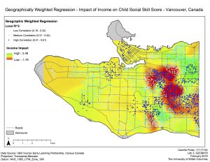
Map 1 (Appendix A) portrays the GWR results for the predicted local impact of income on the child social score skill as it varies over the enumeration areas of Vancouver. The areas in red shows where the variable of income has a negative impact on the social score whilst areas in green represent areas where income has a higher positive impact on the score. The estimated influence results are accompanied by the r^2 values of the GWR analysis, which show the 3 levels of correlation, or the levels of “fitness” of the predicted model compared to the observed values. Areas with dark blue dots have high correlation, and in such areas it can be said that the GWR model worked well. On the other hand, areas with light blue dots have a lower correlation and fit the model less accurately.
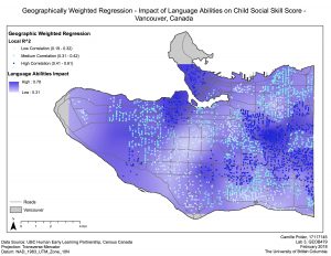
Map 2 (Appendix A) shows the local impact of language abilities on child social score. Areas with dark purple represent areas where language abilities have a higher positive impact on the score. Light purple areas represent spatial locations where the impact of language abilities is still positive yet less strong. R^2 values, seem to indicate that, like the income predictions, areas with higher positive impact have a more positive correlation between the estimated model and observed values.
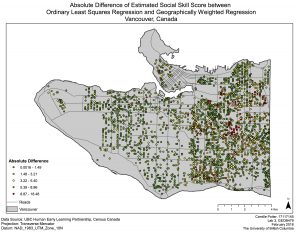
Map 4 (Appendix A), shows the absolute difference between the estimates of the social skills scores calculated from the OLS and the GWR. It is possible to observe that areas with the biggest difference between the regressions’ prediction are in East Vancouver. This implies that where the absolute difference is the biggest, the OLS regression was least successful in predicting the social skill score. A possible explanation for this is that for those feature with high absolute differences, the OLS global model may have failed to account for geographic variation and for the impact of neighbors around the features. Furthermore, by looking at the average of the predicted social scores by the OLS (77.26/100) and GWR (78.98/100) and comparing it to the average of the observed values (78.86), it can be seen that the GWR’s predictions were more accurate than those of the OLS. Hence supporting the fact that the geographically weighted regression model is a more accurate predictor of the relationship between the dependent variable and the independent variables as it varies over the study area.
Several conclusions were made from the report:
The geographically weighted regression is a spatial extension of aspatial regression. Unlike an OLS, this regression goes beyond generating a global model and estimates local predictions of relationships between the independent variables and the dependent variables by considering the neighbors around each field within the area of study. GWR is useful in evaluating spatial heterogeneity across landscapes to model relationships such as health problems and the impacts of a range of socioeconomic variables on such issues; GWR often leads to higher r^2 values/higher fitness of the model and its output and predictions are more accurate.
Full lab: lab3