When I first read the module for this week, I thought to myself that this week’s task may go relatively smoothly; I was so wrong! Even with my comfort level in math and science, I was perplexed with simply how and where to begin. One of the main frustrations in navigating the Palladio file was how the facet dimensions were labeled in a non-sensical framework; Id, Id_1, Id_2, etc. Clearer identification of labels and facets would have eased the process immensely, as I resorted to systematic clicking through each target to best understand how each graph changed as a result of changing the base variables. A second frustration concerned how limited I was not able to individually select data and change its position/orientation in space; when I pulled on one data point it often grabbed the entire web of networks and moved in the same amount and direction. On top of the difficulty of analyzing the data, another important consideration is how limited the data really is; the data that is available consists mainly of the track title, student name, and some descriptive statistics of how many times it was selected. The task of determining the reasons for similar responses, or capturing the reasons behind the choices is, in my opinion, simply too large for the small amount of data that is provided. Helpful data could have included general data demographics such as the respondent’s sex, age, preferred pronouns, etc., in addition to contextual data demographics such as musical background, current musical tastes, and musical aversions, etc.
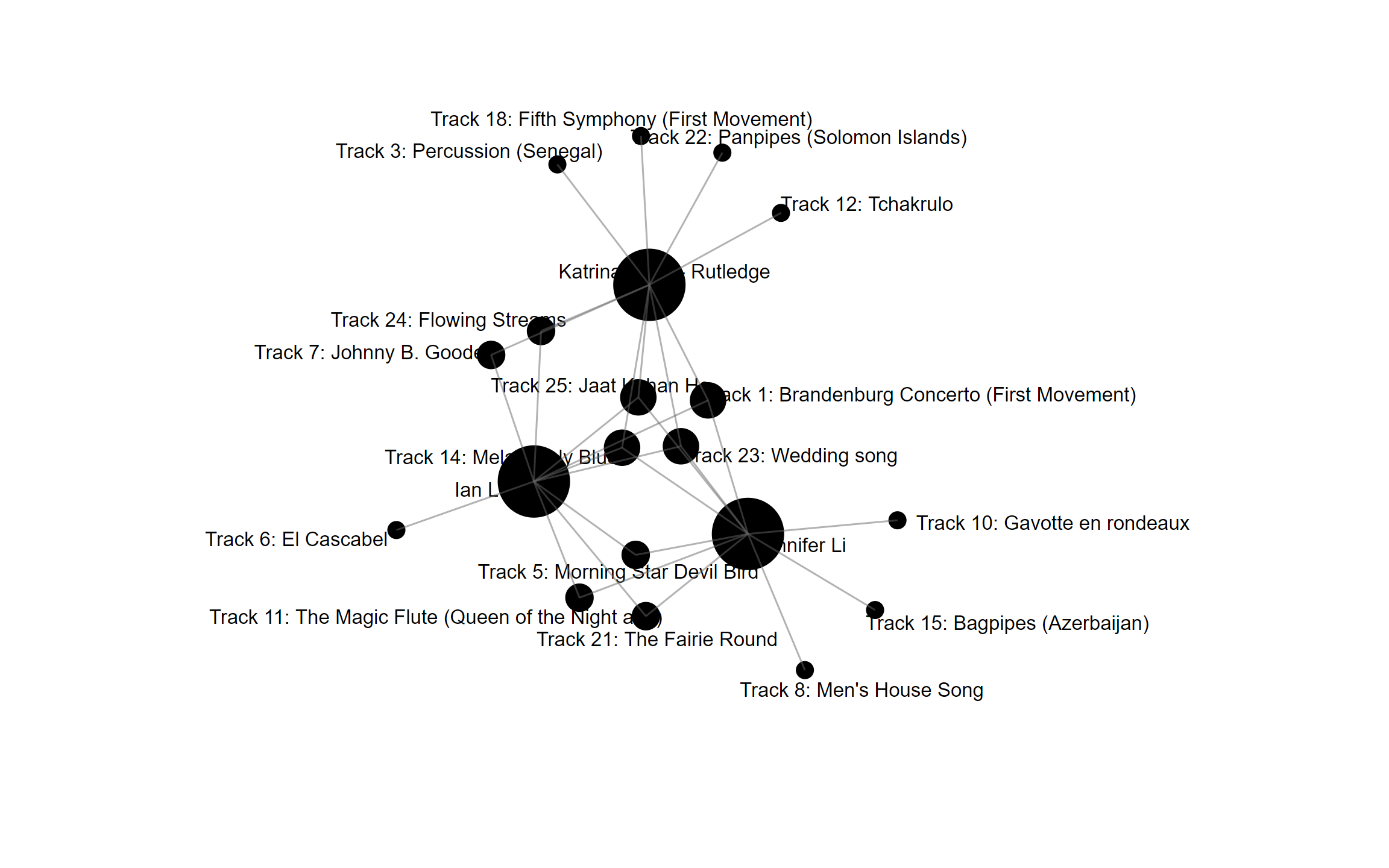
I decided to begin with commonalities, much like most programs which use AI programs to offer friend suggestions based on your personal data, online behaviour, (and even offline behaviour when your microphone manages to listen to what you’re saying!). Although I mentioned that I wanted to start with commonalities, I really did not know where and how to begin. As I alternated through various choices, I found a common theme between myself and two other students: Jennifer Li and Katrina Wong-Rutledge. This graph highlights 4 points of intersection between the 3 of us: Track 1, 14, 23, and 25. I also shared 2 additional points of commonality with Katrina and 3 additional points of commonality with Jennifer.
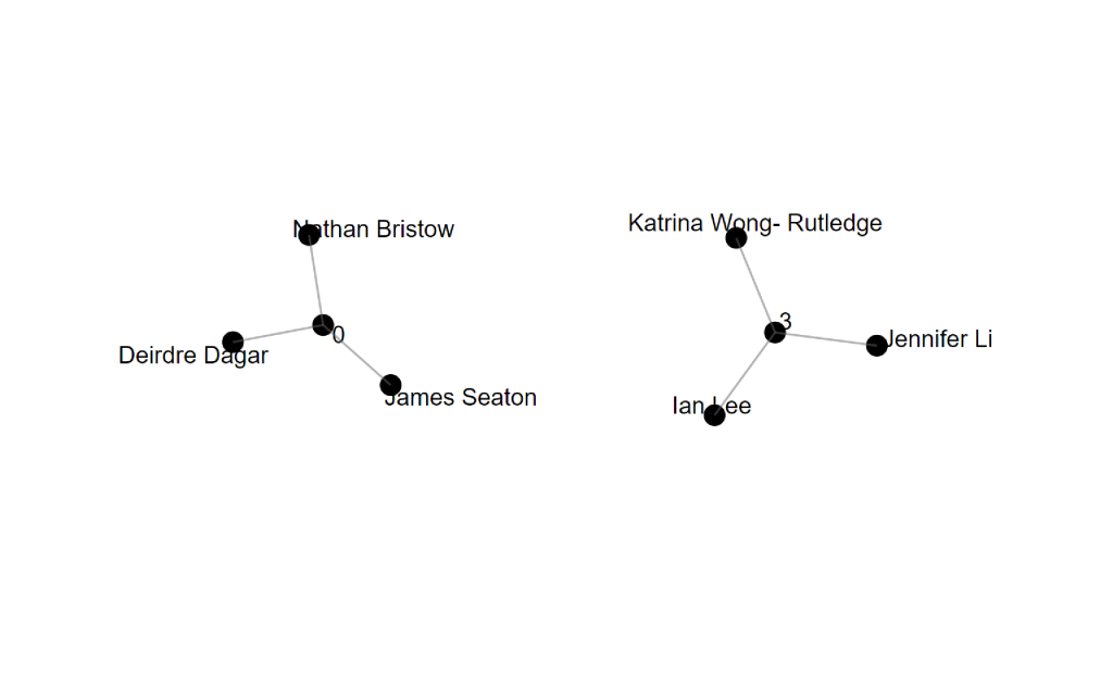
The difficulty in interpreting this graph again returned to the confusion regarding the variable’s designation of “Modularity_Class”. My first thought was that it referred to points of intersection, but that clearly made no sense as ‘0’ was a result for a group of three: Nathan, Deidre, and James. Likewise, when selecting the modularity_class for myself, Katrina, Jennifer and I are in group 3, which also doesn’t match our 4 points of intersection. Frustrating!
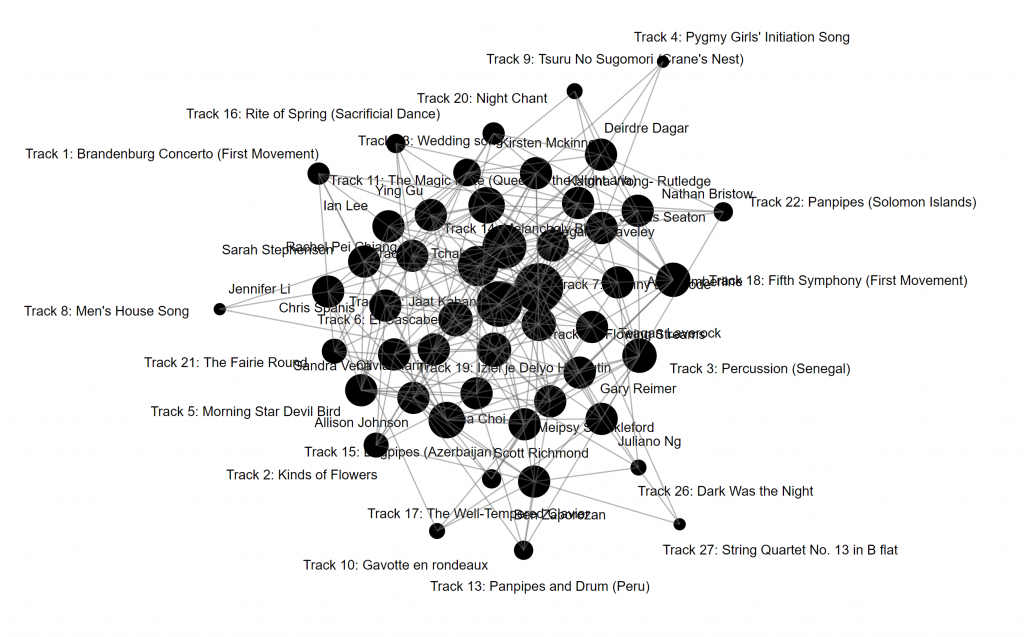
A decisive step occurred partway through my hair-pulling when I decided to reverse the Source of the graph to be the Track #, and the Target of the graph to be the student (source). Amidst the chaos, I selected that the side of the node would depend on the number of commonalities, and thus realized that the following graph displayed the most popular track as the largest node and the least popular track as the smallest node:
And so, I started my journey in the reverse direction using the graph above. I noted my personal choices: (#1, #5, #6, #7, #11, #14, #21, #23, #24, #25), and removed the other tracks from the chaos. At this point, the source table became a valuable resource as I was able to determine the actual number of points of commonality with each student: the highest number of intersecting points was 7 of 10, and the lowest was 3 of 10. The most shared points of commonality was with 1 student (7 point): Jennifer, followed by 5 students (6 points): Ying, Selina, Rachel, Megan, and Katrina. I decided to remake the graphs focusing on these 6 students:
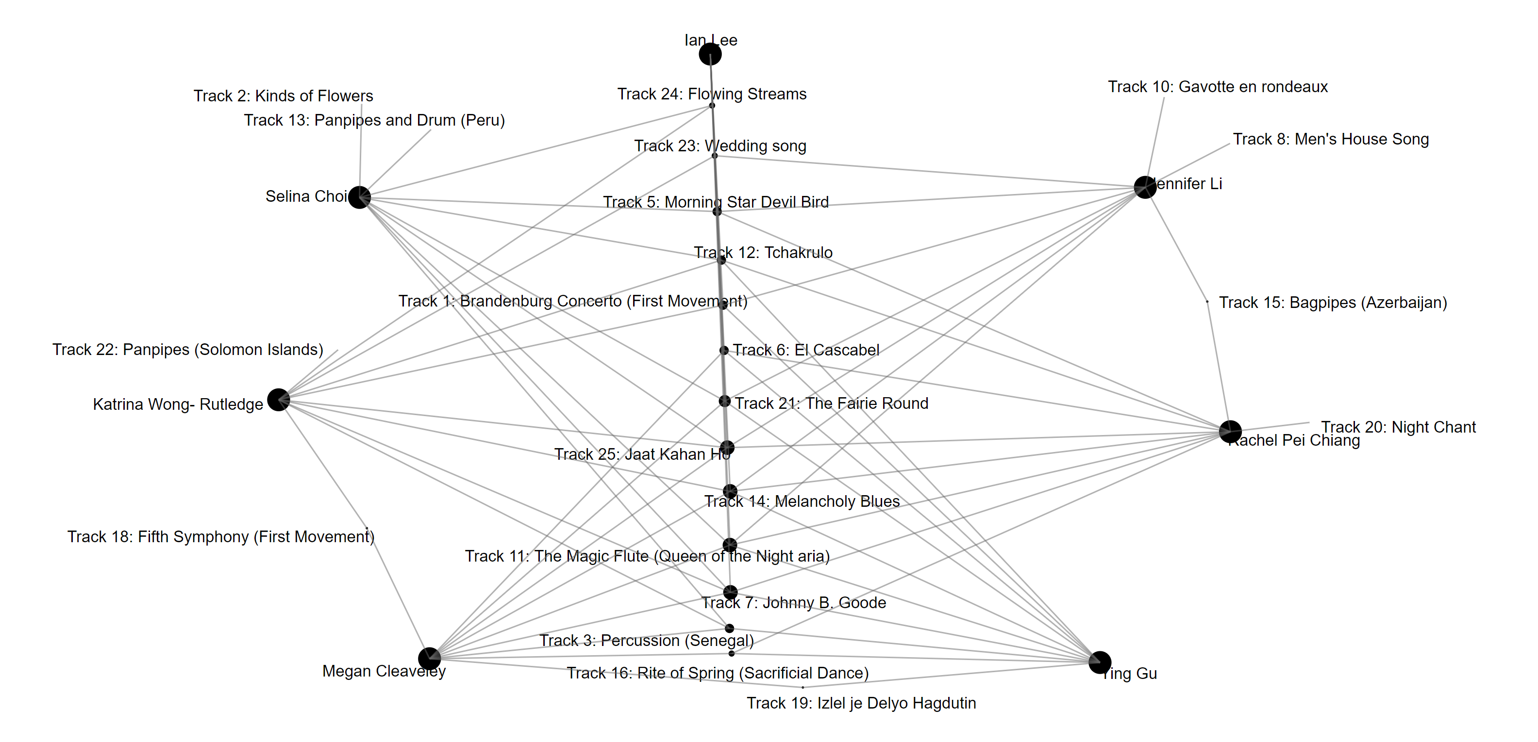
By rearranging the common tracks to be the ‘spine’ of the graph and arranging them by size with the most popular at the bottom and the least popular at the time, I finalized this graph by placing the students on the outside edge. I was able to identify the strongest point of commonality to be Track 7 and Track 24 being the weakest.
Assigning this role to an AI algorithm is likely the logical choice for applications that seek to make connections between given parameters. For a social application, networking sites would benefit from this use as it would strengthen connections between existing members, suggest commonalities, or even recommending new connections to further the complexity of the interconnected figurative web. For a medical application, this may benefit tracing sites for points of contact in reversing back time to find commonalities, and thus, a source of interest such a contaminated source, or a point of infection. For dating applications, this would likely be another source of suggesting best matches by selecting high degrees of commonality while disregarding others with low degrees of commonality. For business applications, data could be tailored to ‘suggest’ similar material to further entice consumers to spend on additional products, while shelving other products that are likely to not be interesting. As the enticement to make profits based on consumer interest would be a huge draw, it is no wonder that data mining companies would purchase consumer data from as several different sources. To benefit further from this application, it would likely suggest that the more information you feed into the algorithm, more accurate the results would be. For us students in ETEC540, we simply offered our names and our top 10 choices with less else to distinguish who we are. I believe that additional data points would increase the complexity while refining the list of commonalities between all of us.
On a final note, I found it most interesting that the students that I also shared the most commonalities with have recognizable Asian surnames; although it may mean little due to the limited information, this would be a good place to start with more data from our class set. In a reversal of data, the strategies that I employed to find commonalities could be used to find differences, starting with my peers who had the least amount of commonalities, and identifying key characteristics that could be distinguishing factors.