Week 4 began with the topic of geography and health. As I’m sure is quite apparent, geography is intrinsically linked to health in many ways. For example, the environment we live in, the people we are surrounded by, and our demographics all influence our health. Some individuals are located in more polluted regions, while others have less access to health services. As the population is growing and the climate is changing, it is becoming even more important to understand the linkages between these two topics, and how we can use this information to our advantage.

We spent this week talking about two kinds of geography: medical geography and health geography. Medical geography is the application of geographical perspectives and methods to the study of health, disease, and health care. This concept has been around for centuries, but it really took off in the 16th century. Due to the strong activity of the military in the 18th century, medical cartography emerged. Prior to the 1950s, medical geography was led by physicians as they had a good grasp of the disease in question. However, since the 1960s, geographers have taken over the field. Medical geography is seen as an integrative, multi-stranded sub discipline of geography, however, it comes from very colonialist roots.

Health geography also looks at local variations in health status and health care provisions, but also looks at the access to, location, and utilization of health facilities. It has two main approaches: Traditional, which accepts diseases as naturally occurring and culture free, and Contemporary, which adopts the stance that notions of health, disease and illness are problematic and are ultimately linked to power relations within a society.

While similar and absolutely linked, these two sub-disciplines are both extremely important to understanding geography, health, and all the connections they share.

Week 3 was spent continuing on Lab 2, which analyzed the changing landscape of Edmonton between 1966 and 1976. However, during lecture we dove into some key concepts relating to landscape ecology, mainly focusing on abiotic conditions and biotic interactions.

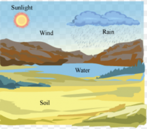
Abiotic conditions, such as climate, topography, and soils, play a large role in what plants and animals can live within an ecosystem as well as how well they prevail. For example, constant weather patterns and conditions form the climate in which flora and fauna are expected to live. Heavy rains allow some species of plants to grow while excluding others that flourish under drier conditions. Topography also plays a role in climate (i.e. the rain shadow effect), but can also impact other disturbances. For example, wildfire moves more easily uphill.

Biotic interactions impact each other (i.e. species), but also the environment they live in. Competition within and between species forces patterns to emerge within landscapes. On top of competition, there lies species that are so important in an ecosystem that without them the ecosystem could collapse. These are known as keystone species and every ecosystem has one. As humans, knowing the way in which these landscape patterns occur is crucial so we do not damage them beyond repair, such as through removing a keystone species.

Week 2 focused on geographic and landscape metrics such as patterns, processes, and scale. We discussed some issues between pattern and scale, which is deemed the central problem in ecology. As there are different spatial and temporal scales, as well as different ecological organizations, it is very difficult to decide at what spatial and temporal scale an ecological phenomenon should be studied.

Due to the geographic nature of the software, GIS almost always maintains some level of spatial autocorrelation. That is, if the presence of some quantity in a sampling unit makes its presence in neighboring sampling units more or less likely, that phenomenon exhibits spatial autocorrelation. This is contrary to spatial statistics, which assumes that everything is random.

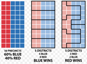
One particular way that spatial autocorrelation exhibits itself is through MAUP, or the modifiable areal unit problem. This problem arises when different areal arrangements of the same data produce different results. One example of MAUP in the real world that I believe is quite relevant in todays day and age is gerrymandering. The figure below exhibits this phenomenon perfectly. Depending on how governments divide census units, they can in essence force an election to go in favor of Democrats or Republicans.

.

During analysis, a spatial analyst must be extremely careful in how they approach MAUP.