Preliminary Research:
A key factor in our study was choosing representative vehicles to develop a most practical route between the University of British Columbia at Vancouver and the University of Toronto. We decided to compare the feasibility of using a standard gasoline-powered car (Pontiac G6), a hybrid vehicle (Chevy Volt), a standard full electric car (Ford Focus), and a higher power, full electric car (Tesla Model S) to complete the journey. It was also important to consider how we would obtain the spatial data for the electric vehicle charging stations, which is shown in the Data tab.
Within ArcGIS:
Data Input
For each province, the road network data (CARTO) was narrowed down to expressways, principal highways, secondary highways and major roads using a definition query to select only these attributes. The queried data was exported as a new layer in the geodatabase. The Merge tool was used to combine the road layers from the different provinces into one layer so the route would not stop at provincial boundaries.
Charging station locations were inputted into ArcGIS manually by adding in point data for each charging station to create a charging station layer. Some charging stations that were very far North or in highly concentrated clusters (ie. Vancouver area) were not included because it was deemed unnecessary. Charging stations were separated into three separate layers based on their charging level (1-3). Buffer zones were created around each charging station for the various distances that each of the electric vehicles could travel (85km for hybrid Chevy Volt, 122km for electric Ford Focus and 507km for electric Tesla).
It was assumed that there would be sufficient gas stations along the way for the gasoline powered vehicle ensuring the shortest distance route would be the most practical route.
Network Analyst
A network dataset was designed to create the travel path from UBC to UofT. Connectivity rules and network attributes were defined for the network dataset using the shape length (meters) and travel time (min) attributes from our data. The network analysis allowed the road data to be treated as roads in ArcGIS. The network was rebuilt for each vehicle in order to incorporate the unique friction values into the route specific to that vehicle.
Assigning route values
Friction values were assigned to the polyline sections of roads that were within the buffer zones of charging stations.
Level 3 charging station polylines = Friction value 1
Level 2 charging station polylines = Friction value 2
Level 1 charging station polylines = Friction value 3
Lower friction values were favoured to represent preference for a faster charging station.
Friction values were assigned to the major roadways that were used.
Expressways = Friction value 1
Major Highways = Friction value 2
Secondary Highways = Friction value 3
Major roads = Friction value 4
Friction values were combined using a field calculation:
“CARTO+FRICTION_XX” (roadway friction values + charging station friction values)
Each vehicle used a different field calculation depending on the distance that the vehicle could travel on a full charge.
Friction values were incorporated into the route as a hierarchy. The route was drawn to minimize travel time while favouring sections of road that were at the top of the hierarchy (the lowest friction values).
Service Areas – data check
Additionally, service areas for each charging stations were created to account for travel time rather than just distance, which is the case with buffer zones. In order to create these service areas, we first had to determine the average travel speed for the route between Vancouver and Toronto. We calculated the average travel speed to be 90km/h by rounding the average speed limit of polylines to the nearest 10%. The maximum travel time that each electric and hybrid vehicle could go in between charges was determined with the following equation:
(1/Average speed)*(Hour to minute conversion)*(Max distance)
Chevy Volt: 57mins Tesla: 338mins Ford Focus: 80mins
Unfortunately, the service areas were not as effective as we had hoped as they are not usable with features outside of the network analyst. Specifically, we could not “select by location” within the service areas which we needed to do in order to assign the friction values. Instead, we used the service areas as a visual comparison to assess the accuracy of the buffer zones, which represents a constant distance in all directions. Buffers do not account for travel time or calculate the distance along the roads because they exist outside of the network. Buffers were used instead of service areas because of their ability to work with the other features in the analysis.
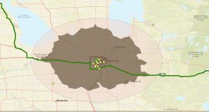
Figure 1. shows a comparison of an 85km buffer zone and service area. Each method returns a slightly different result, which was taken into account when drawing conclusions.
Route development
The route was drawn using the Route feature of the Network Analyst. We inputted the start and end locations manually and allowed the program to draw the route between them. We configured the route calculator to choose the route along the roads with the shortest travel time while choosing segments of road with the lowest friction values. As a result, we had to rebuild the network and redraw the route for each car to account for the different friction values incurred from having different ranges. The fastest route was then determined for the gasoline powered car by ignoring the friction value hierarchy altogether.
When determining the amount of days required to make these routes it was assumed that driving would be conducted non-stop, in shifts by multiple drivers.
Calculation of Travel Time
The amount of time that it would take to travel along each route without stopping was calculated with a route analysis to find the total travel time for the route. This feature adds up the time travel attributes for all of the polylines along each route. Since resting time was not incorporated into this study, travel time was the total travel time for the gasoline powered vehicle. For the electric and hybrid vehicles, charging time was incorporated into the calculation by adding 5 hours to the travel time for each level 2 charging station and 0.75 hours for each level 3 charging station stopped at along the way. Lastly, the total travel time for each vehicle was converted from hours to days.