
To identify core habitat areas, we first needed to assess overall habitat suitability in our project area. According to the literature (Cleland, 2013), the following factors were to be included in such an analysis:
- Prey density (our prey capability raster)
- Forest Service Road (FSR) density (ideal being less than 0.42km/km2, worst being more than 0.62km/km2)
- Wetland presence
- Urban areas (constraint)
- Main roads (constraint)
For prey density, we used our prey capability raster. For logging road (FSR) density, we input our active FSR layer into the ‘Line Density’ tool to create a raster showing the the density of active FSRs across the landscape (km/km2); we then reclassified the raster so that density values were divided into 3 classes, number 3 being the most ideal (less than 0.42km/km2). The wetlands layer was converted to raster and reclassified to Boolean values, with 1 indicating wetland presence. Urban areas and main roads were buffered by 1000m and 250m respectively, then also converted to raster and reclassified to Boolean values with 0 indicating the presence of the constraint. Each layer was trimmed to the project boundary.
A weighted sum was conducted to produce the wolf suitability raster, in which prey capability was given a higher weight than FSR density and wetland presence, and urban areas and main roads were given negative weights. This produced the following raster layer (Figure 3), with the least suitable areas in red and the most suitable areas in blue.
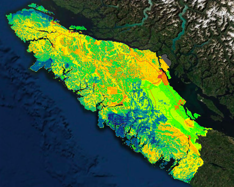
Figure 3. Vancouver Island wolf habitat suitability raster, with the most suitable areas in blue (cooler colours) and the least suitable areas in red (warmer colours). This makes sense, as many of the favourable areas are in protected areas (even though this layer was not used in the analysis) and the least favourable areas are urban areas and roads.