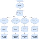
The first step of our analysis was to create a kernel density map for each type of crime in the city of Chicago. These maps display hotspots of crime throughout Chicago on a city wide scale, which will prove useful later on in the analysis. The flowchart below is a visual representation of the steps that were taken. Also provided is a table displaying the total number of offenses for each crime type.
| Type of Crime | Total Number of Offenses |
| Narcotics | 11,646 |
| Robbery | 12,056 |
| Criminal Damage | 30,813 |
| Homicide | 773 |
A fuzzy mode and hierarchical nearest neighbour analysis were performed next using the program CrimeStat. We chose to include this step in our project because these two spatial clustering tools identified hotspots of crime at a local level compared to the kernel density which was a city wide analysis. With the clustering of crimes identified at a local level we could compare those to the locations of the crime attractors providing further insight for our research. With maps comparing the fuzzy mode and hierarchical nearest neighbour analysis complete, we began to focus on train stations and sport stadiums. To do so we needed to normalize our data by obtaining a number that represented the number of offenses of each crime type per meter squared. A total number of crimes was obtained for each type of offense, which was then divided by the total area of Chicago. Our results are displayed in the table below.
| Crime Type | Calculation (Total number/M^2 of Chicago) | Crime incidents per M^2 |
| Narcotics | 11,646/597,460,691 | 0.0000195 |
| Robbery | 12,056/597,460,691 | 0.0000202 |
| Criminal Damage | 30,813/597,460,691 | 0.0000516 |
| Homicide | 773/597,460,691 | 0.00000129 |
With the average offense per meter squared in hand a proximity analysis of the crime attractors was performed. This was done by creating a multi-ring buffer around both the train stations and the sport stadiums. For the train stations the buffers were set at 100 meters, 250 meters, and 500 meters. For the sport stadiums the rings were set at 250 meters, 500 meters, and 1000 meters. The buffers were made larger for the sport stadiums because there are far fewer of them in the city and because they attract far larger crowds so crimes committed by fans may occur some distance from the structure. Next we performed a spatial join between the buffers and the four types of crime to see how many offenses occurred within each distance interval. Flowcharts were created to visualize these steps and they provided.
The final step was to calculate the offenses per meter squared within each distance interval of the buffers surrounding the train stations and sport stadiums. This was done by dividing the total number of offenses in each distance interval by the total area covered by each buffer ring. The results allowed for a comparison to the average offense per square meter throughout all of Chicago, if the numbers were greater in the buffers it could be indicative of a crime attractor. The number for the average offense per meter squared in the city is provided in the following tables where all of the results can be seen.
Calculations for Train Stations:
| Crime Type | Offenses per M^2 in 100m Buffer | Offenses per M^2 in 250m Buffer | Offenses per M^2 in 500m Buffer | Average Offenses per M^2 in city |
| Narcotics | 0.0000647 | 0.0000323 | 0.0000264 | 0.0000195 |
| Robbery | 0.000173 | 0.0000509 | 0.0000329 | 0.0000202 |
| Criminal Damage | 0.000136 | 0.0000904 | 0.0000751 | 0.0000516 |
| Homicide | 0.00000235 | 0.00000151 | 0.00000155 | 0.00000129 |
Calculations for Sport Stadiums:
| Crime Type | Offenses per M^2 in 250m Buffer | Offenses per M^2 in 500m Buffer | Offenses per M^2 in 1000m Buffer | Average Offenses per M^2 in city |
| Narcotics | 0.0000102 | 0.00000637 | 0.00000711 | 0.0000195 |
| Robbery | 0.0000331 | 0.0000149 | 0.0000236 | 0.0000202 |
| Criminal Damage | 0.0000369 | 0.0000400 | 0.0000485 | 0.0000516 |
| Homicide | 0 | 0.000000212 | 0.000000484 | 0.00000129 |


