Random forest models are more commonly run directly with R or Python than from within a GIS environment, but there are implementations available for working spatial data sets. Our course primarily uses ArcMap, but its implementation is quite limited in applications, and seems to be designed specifically for image classification. GRASS GIS, on the other hand, has two options for implementing a random forest model that are suitable for ecological modelling: interfacing with R and the r.learn.ml add-on invoking Python’s scikit-learn toolkit (Pawley, 2018). The latter can be run directly from a GIS interface, so this method was chosen for its relative simplicity.
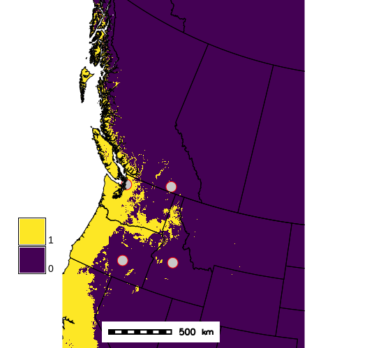
Creating and validating a model with a large spatial extent, about 1000 training points and 30 input parameters proved to be computationally expensive, thus a subset of parameters was selected from the inputs based on two test runs. In the first test run, a smaller sub-section of the study area was considered (the rectangle shown in the above image) with all input parameters. This area was chosen as it contained a representative subset of training data. The first test provided information about the most predictive inputs, however many of the variables that should have been predictive based on literature were not found to be important, and the initial run had a low accuracy of 79%.
For the second test model, parameters related to soil moisture, frost tolerance and snow, such as number of frost free days and winter precipitation, were added based the habitat requirements of A. macrophyllum (Fryer, 2011). The second test included 18 variables and was run over the entire study area. This test had a higher accuracy, and 11 variables were selected from this test that had the highest importance scores: aspect, beginning date of the frost-free period, mean annual precipitation, mean temperature of the coldest month, mean summer precipitation, number of frost-free days, temperature differential (difference between warmest and coldest month), July maximum temperature, January minimum temperature, topographic wetness index and winter precipitation.
The final model using 11 climate and topographic variables was built for the baseline climate period, including 10-folds cross-validation for accuracy assessment. This model was used to predict A. macrophyllum distribution for the 2050’s and 2080’s time periods. Three different ensemble climate models were considered for each time period, which are derived from a number of individual climate models for each emission scenario (Hamann, 2013). This report primarily considers the moderate emissions scenario (A1B), but also compares these results to projected distributions under high- (A2) and low- (B1) emissions models.