Data Used
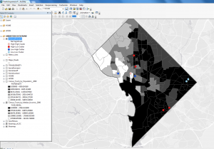
All data was acquired from the Washington D.C open data catalogue unless otherwise specified, with exception of the base map of D.C which was retrieved from within ArcGIS.
- Basemap of D.C (ArcGIS)
- Roads (All)
- Metro Stations
- Metro Lines
- Sex Offender Registry
- Crime Incidents in 2017
- D.C Boundary line
- Census Tracts by Median Income-2000
- Census Block Groups by Population Density-2000
- Address Points
Works Cited
Downs, J. A. (2016). Mapping sex offender activity spaces relative to crime using time-geographic methods. Annals of GIS, 22(2), 141-150. doi:10.1080/19475683.2016.1147495
Patterson, Z., & Farber, S. (2015). Potential path areas and activity spaces in application: A review. Transport Reviews, 35(6), 679-700. doi:10.1080/01441647.2015.1042944
Methodology
Attribute Tables
The data acquired from the D.C open data was complete but was unnecessarily detailed for the scope of this project. In particular, the data pertaining to the sex offender registry and 2017 crime incidents had details which were not needed. Therefore, the first step in terms of analysis was the filtering of data in order to create a more appropriate data set. As this project was aiming to examine sex offenders and sexual assault crimes I filtered the crime incidents in 2017 to only include violent sexual assault crimes. This led to a total of 291 crimes for the analysis. In turn, the overall amount of sexual offenders was reduced. This was a crucial step when preparing to conduct analyses of activity spaces and potential paths as only offenders with both a home and work addresses would be suitable. The reasoning for this is due to the creation of anchor points and travel between two areas. Though D.C requires that all sex offenders give home and work addresses it was not the case that each offender had both of these, possibly due to living outside area boundaries or not having jobs within D.C. Therefore all offenders which could not form a pair from both home and work addresses were deleted. Moreover, I chose to not account for school addresses due to the small size of offenders which had these. In creating the final offender table I filtered by work and school and created two tables based on this. I then recombined the separate tables based on a combination which used four columns (last name,first name,FID and objectoid) in order to ensure the maximum likelihood of names being matched correctly. This resulted in 275 pairs been created.
Address Locator and Geocoding
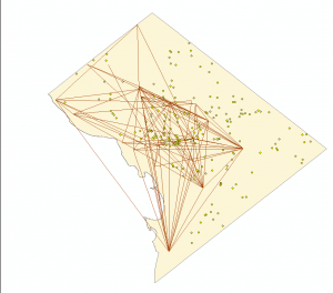
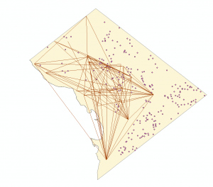
In order to map potential path areas through the use of lines the xy to line tool was needed. Though the attribute attribute for crime incidents (which were not being mapped in this fashion) had x,y coordinates the sex offender pairs attribute table was devoid of these. Therefore it was necessary to create x,y coordinates for the attribute table. Though the obvious step would be to geocode the addresses which were present in the sex offender table this repeatedly created x,y coordinates which were inaccurate. Instead I first created an address locator using the reference data(Address points) downloaded from the D.C open data. The reference data included x,y cords, zip codes and detailed street names. In total i created four address locators which all used different styles. The locators created were : Single House,One Range, Street Name, Zip 5-Digit. The locators which were made for single house, one range and street name were not completely suitable due to differences in the way which the Address Points reference attribute table and the Sex Offender attribute table were written. Therefore I decided upon using the Zip 5-Digit address locator. This decision in turn would lead to the largest amount of uncertainty throughout the project and significantly affected the results of the sex offender lines, though I do not believe this negated all the results. Upon creating the address locator I was able to geocode the the sex offender pairs and in turn form x,y coordinates which I then created lines from using the xy to line tool. The result of this can be seen below in which left is overlaid onto work addresses and the right is an overlay of home addresses. Though to an extent some of the issues are obvious at first glance- the overall uncertainty of these lines will be noted in the discussion.
Statistical Analysis
Though not a large interest to the scope of the overall project it is still undoubtedly important to run test statistics in order to examine how the data of interest is present through the study area. In order to do this I produced a series of spatial auto correlation reports all of which can be seen on the Statistics Page.The statistical reports which were produced detailed average nearest neighbor, optimized hotspot analysis and both global and local Moran’s I.
Kernel Density
Not all crimes occur equally spatially or temporally. Therefore it is important to consider when the assault occurs in order to determine weights for the crime. According to the National Crime Victimization survey 63% of all violent sexual crimes (rape and assault) occur during the night time hours, while 37% occur during day time hours. Therefore, as the crime attribute table specified times into three categories, respectively day,night and midnight, I decided to add weights to each of these. As I was unable to find any data which delineated between night and midnight, these categories were grouped for simplicity sake. Therefore a new category in the attribute table was created labeled weights. Day time was given a weight of 0.37, while night and midnight were given the weight of 0.63. These weights would then be used as a substitute for the population field in the kernel analysis. As well I conducted a series of other kernel analyses besides the one on crime locations. Other kernels were created for work addresses, home addresses, and the activity space of the sex offenders.
Anselin Local Moran’s I
The last analysis technique which was used was to create a cluster and outlier analysis of where the violent sexual offenses occurred. This was done in order to determine where, if any, spatial outliers existed. In total 9 outliers were found. They covered categories of low-low (LL), low-high (LH), high-low (HL), high-high (HH). I then overlaid these results ontop of the census data for Median Household income. The result of this can be seen below.