Within the city of Washington D.C sexual assault crimes are undoubtedly clustered. Moreover, it is reasonably to state that the locations of where sex offenders work and live are as well clustered. Lastly, it can be argued that the activity space of sexual offenders is dominantly situated in specific areas of the city.
The average nearest neighbor summary is a highly suitable statistical tool when analyzing how individuals are distributed throughout a city which is defined by a clearly distinct boundary. Furthermore, for similar reasons it can be useful when applied to the situation of crimes. In total four NN analyses were conducted which detailed home addresses, work addresses, both home and work addresses, and crimes. Among all four of the analyses the common trait of significant z scores was present. Moreover, all of the z scores were highly negative (-9.3,-13.0,-15.1,-23.1). Therefore it can be said with a high level of certainty that the occurrence of clustering among all of these phenomenon was not due to random chance. The results of the Global Moran’s I tests as well displayed a similar patter. Though with the z scores of the nearest neighbor analysis this was to be expected. Nonetheless, the Global Moran’s I tests reinforced the result that a significant clustering pattern was occurring.
Knowing that clustering is occurring can be important but it is not overly useful without understanding where and why. Therefore, it can often be beneficial to look at factors which may be occurring throughout a city. Two large predictors of crime are population density and overall income. Therefore census data on these factors can be applied and examined. The two maps below portray census data from 2000. The left shows median income, ranging from the lowest (black) of 0-37619, to the highest (white) of 176560-314301. In turn, the right map details census tracts by median population, once again black representing the lowest and white representing the highest, values range from a low of 0-4300 to a high of 30036-54678.

Image 1-Median Household Income
Image 2-Median Population Density
Of course, the usefulness of the previous two maps is very little without data showing the distribution of individuals. Therefore, it is a better indicator to examine the below images which show kernel results for home and work, overlaid onto median household income.
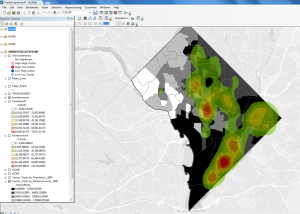
Image 3-Home kernel overlaid onto median household income.
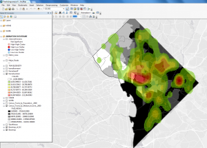
Image 4-Work location kernel overlaid onto median household income.
The two above images both depict similar patterns albeit in different ways. Image 3, which shows the kernel created by home addresses demonstrates significant clustering in the southern portion of the map, with other clusters occurring towards the center. The center cluster can be seen to as well line up quite similarly to the largest cluster of image 4. This is due to the fact that in both situations the clusters are occurring over the D.C downtown core. Moreover, the southern clusters of Image 3 can be noted to be occurring in the census tracts with the lowest median household income. Furthermore, with exception of one lesser area of home residence, it can be seen that no significant number of individuals have household addresses in the northern section of D.C which is as well the area with the highest median household income. Image 4 as well reinforces that clusters are occurring in area of lower income, though it is quite obvious that the overall range extends further across the area of D.C. Nonetheless, the areas of highest income are still showing no signs of a high density of work addresses, while areas of low income still depict high densities.
The next kernel density image which should be examined is where the highest densities of crime are occurring. As already known by the nearest neighbor test and its resulting z-scores, there is a significant level of clustering occurring in regard to sexual offenses.
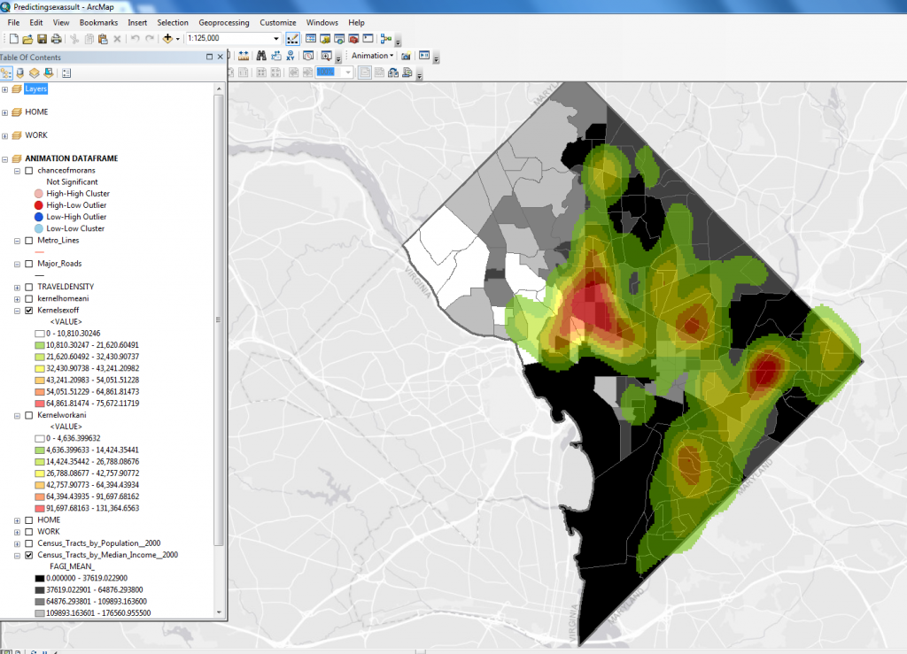
Image 5-Sexual offenses overlaid onto median household income.
Image 5 is interesting for a multitude of reasons. First, it must be noted that image 5 and image 4 line up very similarly to each other. Though the reason for this is unknown there are some speculations which may explain this pattern. First, the largest density cluster which is occurring in image 5 appears to be in the downtown core. This is not overly surprising in terms of crime prevalence as downtown’s experience large amounts of foot traffic and high densities of people, moreover they are generally the travel hubs of a city in terms of bus and train routes. Therefore, to have a high level of crime occurring in the downtown, and having a large number of offenders working in the downtown are not necessarily indicative of each other. Sexual offenses as well follow the pattern which the two previous variables have displayed- that being low densities in areas of high income and high densities in areas of low income. Yet, crime more than the other two factors may be an issue of population density. Therefore, it should be noted that when comparing the crime kernel to the population density map (image 2), areas of the highest crime densities line up with areas that are densely populated. Though an exception to this does occur on the south eastern section of the city. This is due to the fact that the particular area of the city is the Untied States National Arboretum and therefore is not technically populated- though it certainly incurs large amounts of visitors which may explain the prevalence of crime- though this is pure speculation.
Though observing how the variables through kernel density analyses are distributed throughout D.C is important in the overall scope of the project, it is crucial to address the original goal of the project- that being sex offender activity space. I created the sex offender activity space as noted in the methods section through the combination of an address locator,geocoding, xy to line function, and then adding weights and creating a kernel density. The result of this can be seen in image 6.
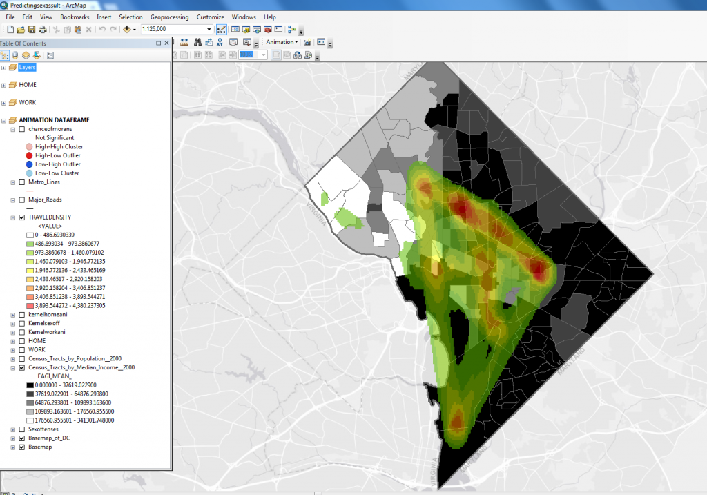
Image 6- Kernel density analysis of sex offender activity space.
Though there are issues with image 6, which will be further discussed in my section on the projects uncertainty, there is still usefulness which can be derived from the preceding image. This kernel was created through lines. Each line was in turn created through the xy function but was done so through been geocoded based on their zip-codes. Therefore, as zip-codes are tied to a specific geographic location similar to addresses all pairs which had the same zip-codes were placed together. This then allowed for the weight to be given based on the occurrence at specific zip-codes. Moreover, as the original lines were calculated based on euclidean distance they are all noticeably straight lines. Regardless, I believe that these results still do depict the underlying activity space which can be expected of sex offenders in D.C based upon their daily travels. Though it may not be as accurate as if the lines were able to originate and terminate at specific addresses, it is still able to show the overall density of where the lines overlay. In turn, the dark red areas of image 5 which depict the most dense levels of crime are markedly similar to where the most frequent travel routes of sex offenders occur. This is in line with Crime Pattern Theory which states that offenders are most likely to commit crimes in areas which encompass the travel paths among anchor points, otherwise known as the activity space between home and work(Downs,2016). Moreover, though it may not be obvious on the above image, the activity space does cross many arterial roads which would likely be used for commuting. As well the activity space has highest levels of density in areas which the metro lines occurs.
Intensity mapping can be a useful tool in terms of predicating the activity spaces of criminals and examining the factors which may influence crime, yet it does have issues. Even though patterns presented above may look similar in many ways- and it is statistically significant that clustering of all of the variables is occurring,it can be dangerous to associate data to a phenomenon. Moreover it is immoral to make assumptions which are not entirely founded based on predetermined factors associated to individuals. Additionally as noted by Downs(2016), the recommitting of crimes by released sex offenders is far lower than criminals who commit other crimes. Furthermore,the high density of sexual offenses committed in areas which the sex offenders home addresses are may not be representative of the sex offenders. Rather, as criminals are generally restricted in terms of employment and therefore pay, this results in individuals with criminal records living in low income neighborhoods. As such, sex offenders are likely in neighborhoods which other criminals (and non criminals) are and therefore the occurrence of most crimes would be higher in these neighborhoods. Similarly this is most likely why the density of home addresses and crime is lower in the areas with the highest median household income. As well, though the activity space of the sex offenders does line up with the sexual offenses for a large part this can simply be argued to be a result of popular travel routes which would be frequented by many individuals who live in the major neighborhoods and commute into the downtown core.Therefore though images 5 and 6 may appear similar in their high and low density areas it is outside of the scope of this project to place whether it is due to the sexual offenders who were analyzed or rather if it is indicative of the general pattern throughout the city.
Uncertainty
The largest factor which influenced the uncertainty of this project was the lines created for the sex offender activity spaces. As discussed above, these lines were anchored to the zip-code points which the work and home addresses existed in. Therefore, though they may have encompassed a large majority of the middle travel space they still did represent the individual addresses. This can be seen below in image 7.
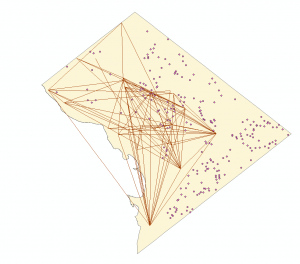
Image 7- Home addresses (left) and work addresses (right) with xy lines formed by zip-codes.
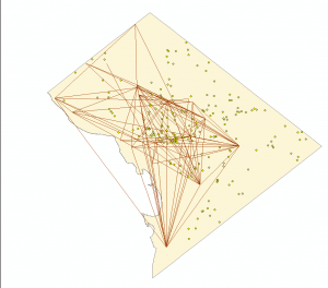
Moreover, the lines visibly cross outside the boundary of the area of study. Though it could be argued that as individuals may choose any way to travel between work and home this is allowed, it nonetheless does not feel appropriate. Additionally, though not represented on any of the above images, D.C has the Potomac River which runs along the west side. This in part is why the south western region often is represented in the census tracts as low income and low population. Though the river does not take up a large section of the map it can be noted in the census data. Furthermore, the lines do cross through this section when leaving from the most southern point in image 7. As individuals likely do not take the river from home to work, this once again is not appropriate when considering the activity space of offenders.
Recommendations For Future Research
- Find better attribute tables detailing street addresses- or filter and rewrite in order to geocode on an address to address basis rather than by zipcode.
- Take into account areas which are likely not to be crossed in an activity space such as large parks,rivers,highways etc.
- Expand on research into potential paths and apply the factor of time.
- Possibly examine a better weighting system for crimes rather than 0.63 for night and 0.37 for day.
- Explore the possibility of adding in schools on top of home and work addresses for the individuals which have addressees.