Lagrange interpolation is a method for finding a function based on (1) the points it must pass through and (2) the goal to find as simple a function as possible.

Since the goal here is to learn the basics of Sage, I’ll only deal with a special case of Lagrange interpolation: in two dimensions, with the number of points to be interpolated to be less than 20 (otherwise, the condition number of the system is huge, and so the answer we calculate can’t be trusted unless we have unimaginably precise data). For this technique to make sense, we also need the x-coordinates of the points to be unique, e.g.,

\(S=\{(x_i,y_i):i \leq 20 \land x_i \neq x_j\ for\ i \neq j\}\subset\mathbb{R}_2\).

We’ll look for a polynomial to interpolate the points. Recall that any polynomial has the form:

\(p(x)=a_0 + a_1x + a_2x^2 + … + a_{n-1}x^{n-1}\).

Notice that for any choice of \(n \in \mathbb{N}\), we have exactly n coefficients \(a_i\). What degree polynomial should we look for? The goal is to produce a system of equations, linear in the coefficients \(a_i\), that has exactly one solution. Given that we have n points \((x_i,y_i)\), it makes sense to choose a degree n-1 polynomial. That way, we have exactly n coefficients [/atex]a_i[/latex], and so our system can at least in principle have a unique solution.

We’ve now defined the system to be thus:

\(
a_0 + a_1(x_i) + a_2(x_i)^2 + … + a_{n-1}(x_i)^{n-1} = y_i
\)

for \(1 \leq i \leq n\). Expressed as a matrix-vector product this is:

\(
\begin{bmatrix} 1 & x_1 & x_1^2 & \cdots & x_1^{n-2} & x_1^{n-1} \\ 1 & x_2 & x_2^2 & \cdots & x_2^{n-2} & x_2^{n-1} \\ \vdots & \vdots & \vdots & \ddots & \vdots & \vdots \\ 1 & x_n & x_n^2 & \cdots & x_n^{n-2} & x_n^{n-1} \end{bmatrix}
\left[\begin{array}{c}
a_0 \\ a_1 \\ a_2 \\ \vdots \\ a_{n-1}
\end{array}\right]
=
\left[\begin{array}{c}
y_1 \\ y_2 \\ y_3 \\ \vdots \\ y_n
\end{array}\right]
\)

Where the matrix whose rows are the polynomials \(p_i(x_i)\) is clearly a Vandermonde matrix, and thus has a non-zero determinant. But this system is exactly what we’re looking for, since for any matrix M, M has a non–zero determinant if and only if there exists a unique solution to \(M\vec{a} = \vec{y}\). So, all we need to do now is find the solution vector \(\vec{a}\)

Finding and Ploting the Solution with SageMathCloud

Head over to the SageMathCloud website to log in.

Create a new project by clicking on New Project…. When the project appears in your workspace, select it, and then click on New and, after entering a name, press the Sage Worksheet. You’ll

Let’s begin by importing a useful library: NumPy. One of the great things about Sage is that it acts kind of like a “staging ground” for the other major mathematical software systems. You can pull in just what you need for whatever project you’re working on. In this case we’ll take advantage of a few functions in NumPy to make finding the solution to the system easy. As the first line at the top of the sheet, put:

import numpy as np

This lets us call a function from the NumPy library by writing np.function_name(...). Now, on the two lines below, enter in the points to interpolate:

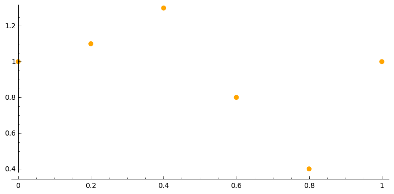
x = [0, 0.2, 0.4, 0.6, 0.8, 1.0]
y = [1, 1.1, 1.3, 0.8, 0.4, 1.0]


Let’s plot the points to see what we’re dealing with. Sage has a useful method, list_plot(...), that takes as a parameter a list of points (as well as any number of customization options) and produces the plot. (Check out this site for more information on plot customization.)

Right now, though, we have two separate lists: x and y. What we need is a data structure of the form \((x_i,y_i)\). Since we’re writing this code in Python, we have access to all of Python’s built-in list capabilities. We can use the built-in function zip(…) to create the list of points, and then produce the plot:

pts_to_plot = zip(x,y)
lp = list_plot(pts_to_plot, color='orange', pointsize=50)
lp.show()

Notice the curious syntax here–we’re creating a graphics object in Python called lp, then calling the function show() on it. You’ll see why this is useful at the end of this example when we produce the final plot.

To execute the code written so far, press Shift-Enter or Shift-Return. Sage evaluates the code and writes the output directly into the worksheet on the following lines. Here’s what the plot should look like at this stage:

Now that we have our target points, let’s evaluate and then plot the solution.

First, we need to create the Vandermonde matrix. We’ll use NumPy’s built-in vander(...) function, which takes in a list of x-coordinates and outputs a Vandermonde matrix of those points, as two-dimensional list (i.e., a list of lists, like [[a,b],[c,d]] instead of [a,b,c,d]):

v_array = np.vander(x)

Now let’s shift gears and start using Sage’s native linear algebra functions. We have our data stored right now as one and two dimensional lists. But, if we transform that data into Sage matrices and vectors, we can use a simple command to find the solution vector \(\vec{a}\) (recall that this vector contains the coefficients for our target polynomial \(p(x)\)):

V_mat = Matrix(v_arr)
y_vec = vector(y)

Now we can evaluate the solution vector \(\vec{a}\) using the backslash operator:


a = V \ y

The backslash operator finds the solution to the system in a computationally efficient manner.

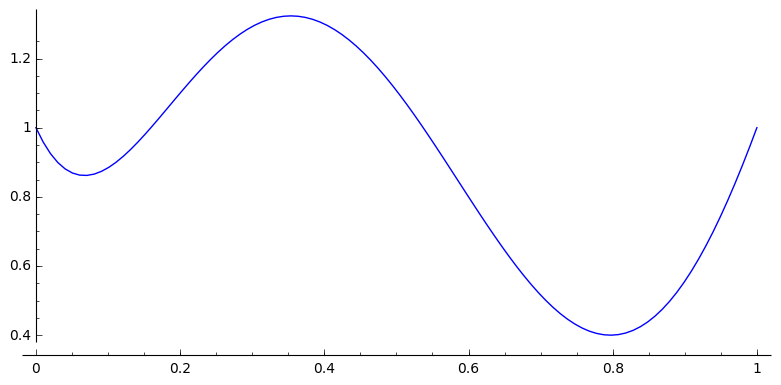
Now that we have the vector \(\vec{a}\) of coefficients, we’ve found the target polynomial. All that remains is to plot the solution. To make a nice looking plot, let’s evaluate the polynomial at 100 evenly spaced points, and then graph those points using list_plot(...).

We’ll use two more functions from NumPy to acheive this task: linspace and polyval. linspace(...) takes in three parameters: a lower bound, upper bound, and the number of points. It outputs a list array containing exactly that number of evenly spaced points between the two bounds. In this case:

x_lin = np.linspace(0,1,100)

gives us exactly 100 points between the lowest x-coordinate and highest x-coordinate. We’ll use another NumPy function, polyval, to find the y-coordinates for each of those 100 x-coordinates. polyval(...) takes in a list of coefficients, the \(\vec{a}\) we found above, and a list of x-coordinates: the x_lin we just found above. Polyval outputs another list containing the solution to the polynomial at each of the x-values in x_lin. These are exactly the y-coordinates we’re looking for:

y_lin = np.polyval(a,x_lin)

Using Python’s handy zip(…) function, we now have everything in hand to plot the solution. Let’s add one more parameter to list_plot, plotjoined=true, to make the plot look nicer. It connects each point on the plot. The code:

lagrange_plt = list_plot(zip(x_lin,y_lin), plotjoined=true, color='blue')
lagrange_plt.show()

will give you the following plot:

To see the two plots together, we can use the fact that Python represents each of these plots internally as objects of the same type. That means we can put them together using the “+” operator:

combined_plot = lp + lagrange_plt
combined_plot.show()


gives the final plot:

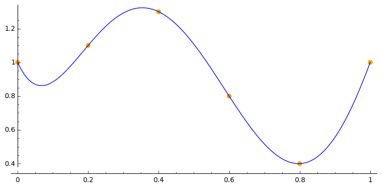
The plot passes through each of the points, as required.