Scale is the main topic described in this week. Because the real world is so complex with so many interactions between factors that we can never find all of them. As a result we often have to decide on a scale that gives a fair representation of what we want to achieve. For example regarding the “marauders” that disturb areas outside their own local scale, should we choose a large scale that includes the marauders’ homes, or should we focus on a smaller scale that gives better representation of the effects within the area of significance? One way of solving this dilemma is to conduct a multiscale analysis, which can give a more complete view of a topic by focusing on factors that are specific to each scale. The problems with scale can be found in many known problems such as the Simpson’s paradox where aggregating data groups change overall results, Modifiable Areal Unit Problem where the same data can produce different results when area is changed, and Ecological fallacy where creating a larger scale can often simplify and misrepresent the details within an area.

The lab for this week used the same processes as lab 1 but uses the city of Edmonton and focuses more on the results produced by Fragstats. We included several additional class and landscape metrics that we deemed to be important. We also created a transition matrix that compared the changes in land use from 1966 to 1976. The transition matrix was much more useful compared to just the two years’ land use areas side by side, because a transition matrix can show us exactly how each portion of land use changed to what. For example with only a simple table we see that non-productive woodland (NPW) areas changed from 19000ha to 7300ha in the ten years, and a logical assumption would be that the 7300ha are the remainder of the 19000ha from 1966. But if we look at the transition matrix, we see that only about 8% of the 19000ha of NPW remained in 1977. It also showed what percentage of other land uses were created from the 1966 NPW, and how the initial NPW changed into other land uses. Effects of scale was also discussed in this lab, where a larger pixel size of 250m looked very different from a 100m pixel map, and many features like river and roads became indistinguishable.

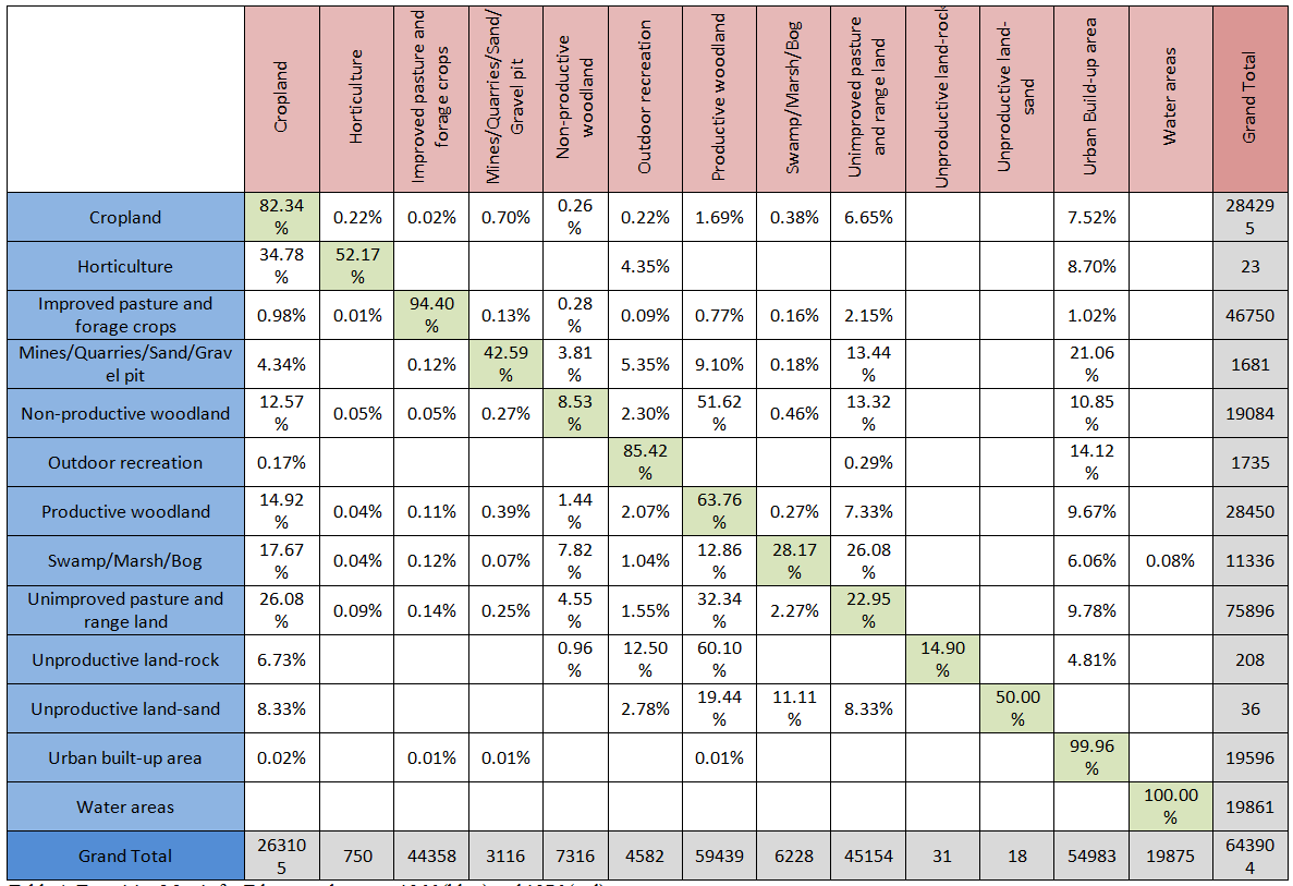
Transition Matrix for Edmonton between 1966 (blue) and 1976 (red)

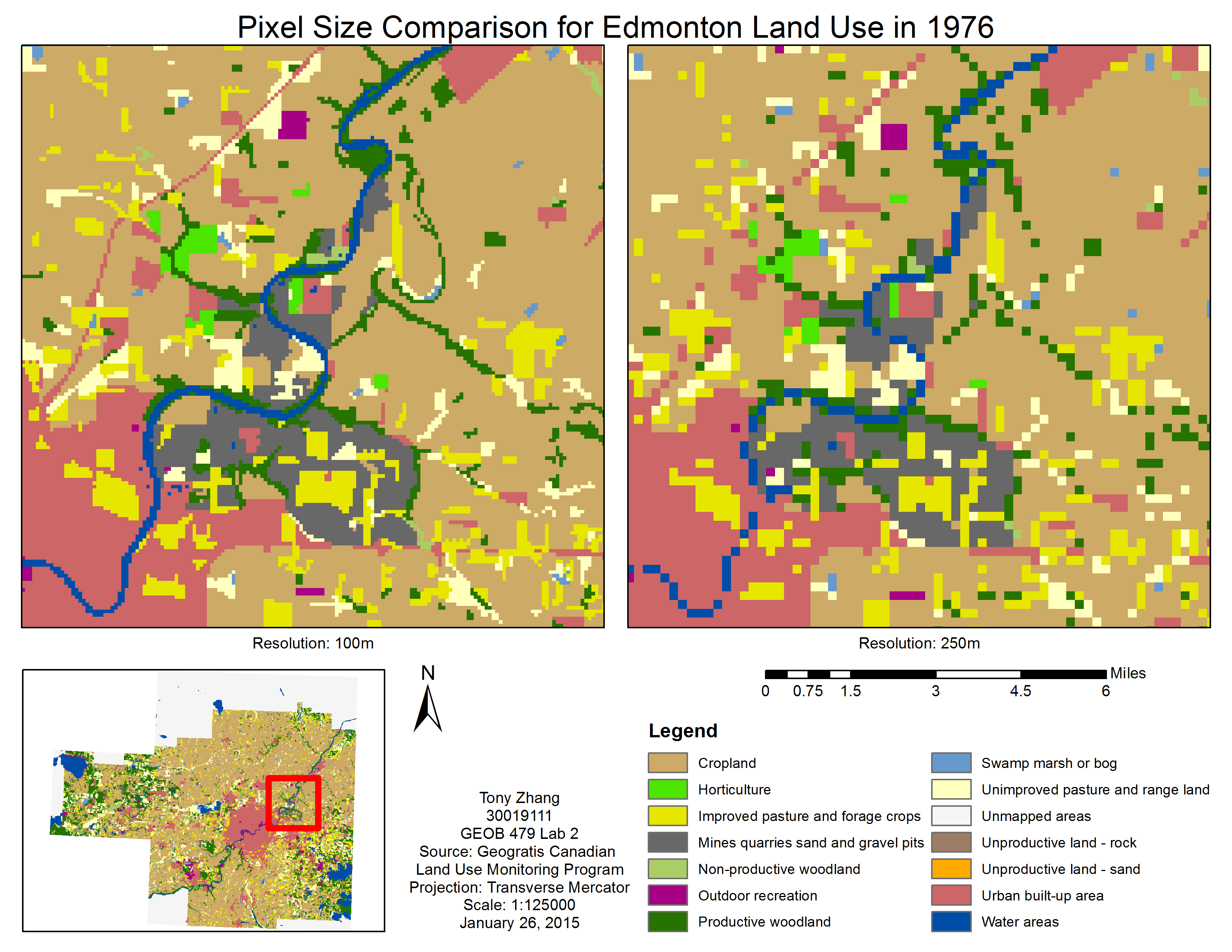
A select portion of 1976 Edmonton Land Use map with raster resolutions of 100m and 250m.

This week we talked about three important but different areas where GIS is important, and they are related through five common themes: patterns, processes, places, people, and perspectives. The first area is landscape ecology, a sub-branch of ecology. Ecology in general is the effects of biotic and abiotic factors on organisms, and landscape ecology focuses more on specifically how the landscape as a factor affects those organisms. Another area is health geography. Health geography is very wide branching, and includes topics like disease ecology, health care delivery, and the relation between environmental and health studies. The third area we discussed is crime analysis. By analysing existing data we can find patterns that help with crime prevention and mitigation. The story about how lead in gasoline was related to crime was interesting, because it showed the impossibility of knowing the complete truth, but analysing data and using statistics can help explain or predict patterns with close enough results despite only having theories for guidance.

We also started working on our first lab which was to help us learn the basics of Fragstats program. Using ArcGIS, we created land use raster files for Saskatoon in 1966 and 1976, and exported it as TIFF files that Fragstats can use. In Fragstats we calculated several class-scale (for each land use area) metrics and a few landscape-scale (whole map) metrics. Determining “edge” depth for each patch was also important for many metrics because it creates different habitats compared to inner areas which cause ecological implications. The resulting metrics can then be exported into other programs like Excel for making comparisons or creating tables and graphs. Below is a sample map for the raster stage of the data in ArcGIS.

Raster map of 1966 Saskatoon Land Use