This week we talked about GIS in relation to crime. This is similar to health geography in that GIS can be used to both map trends and to mitigate/prevent future problems. There are several major criminology theories. The first one is called Routine Activity Theory which is based on the activity patterns of both criminals and victims. For example criminals will more likely commit crimes car thefts at malls than at parks. Another theory is called Rational Choice Theory, which describes that criminals will pick time and place where they are likely to maximize profit and minimize being caught. A third is called Criminal Pattern Theory, which says that crimes will be related to the daily patterns of criminals. These three theories are all part of Environmental Criminology, which focuses on both the spatial distribution of offenders and offences. One way of minimizing crime is through Geographic Profiling, which is to locate and focus on areas of highest crime likelihood. Criminals are also divided into commuters (commit crimes far from home) and marauders (commit crimes around home), and different crimes will likely have different proportions of commuters and marauders. All of these theories and patterns, especially spatial patterns, are used in GIS to help with crime analysis.

We also finished Lab 4 this week, which uses the CrimeStat program for crime analysis. We looked mainly at spatial trends but explored temporal trends too for Ottawa crime data. CrimeStat is able to calculate different kinds of indices relating to distance such as nearest neighbour clustering and Moran’s I correlograms. Moran’s I and Nearest Neighbour analysis is similar, but differs in that Moran’s I looks at the predictability of crime among various regions (Dissemination Areas in our case) while Nearest Neighbour looks at spatial clustering between actual points. Despite small differences, both Moran’s I and Nearest Neighbour appears to show decreased correlation the farther it is from the chosen point/area.

Various methods of identifying crime hotspots were examined. One method we used was Fuzzy Mode, which produces frequency points by analysing crime from its surroundings. One advantage of Fuzzy mode is that it can easily identify hotspots without creating exact areas or points since it samples nearby points. Another method was Nearest Neighbour Hierarchical Spatial Clustering. This method is split between Standard and Risk-Adjusted Nearest Neighbour Hierarchical Spatial Clustering, both of which tries to create ellipses that represent clusters of crime. In theory both methods should be able to create multiple orders, with higher orders being larger ellipses that groups lower orders, but only the Risk-Adjusted version created higher order clusters in our lab. This might be because Risk-Adjusted Nearest Neighbour is normalized rate, while Standard Nearest Neighbour maps absolute crime volume. Another hotspot analysis method was Kernel Density Estimates, which is split between Single surface and Double surface. Single Surface Kernel Density maps absolute crime volume like Fuzzy and Standard Nearest Neighbour while Double Surface Kernel Density maps normalized crime rate like Risk-Adjusted Nearest Neighbour.

Lastly we examined the Knox Index in relation to car theft. This tool looks at both temporal and spatial relations by examining at whether the thefts are close or not close in space, and whether thefts are close or not close in time.

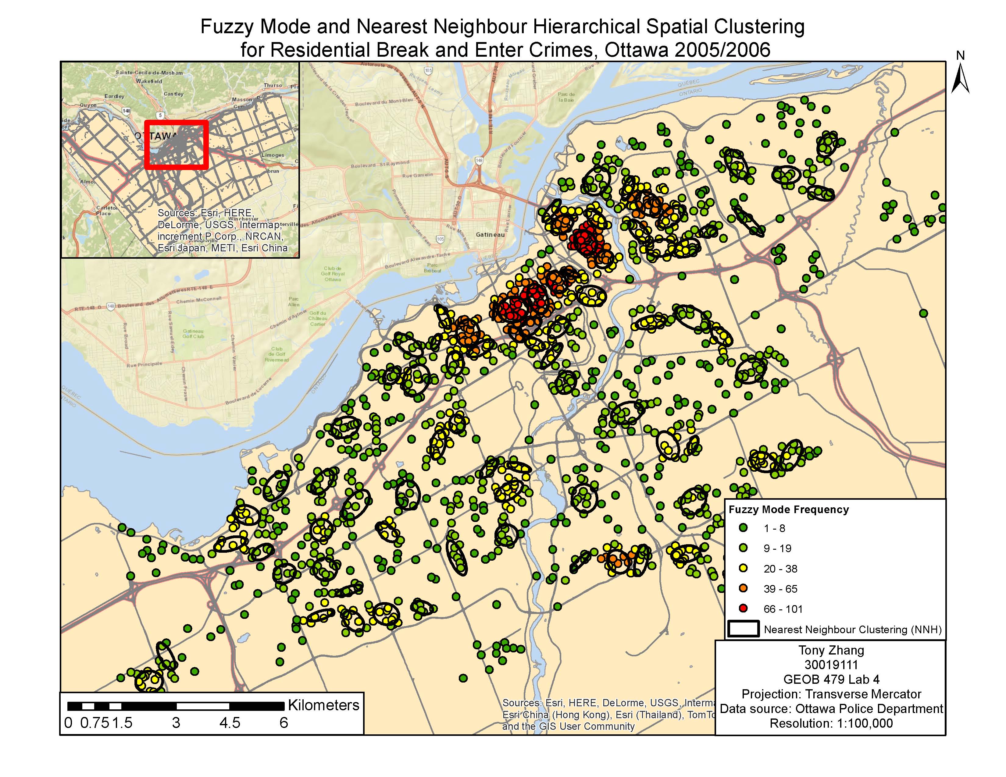
Fuzzy Mode Clustering vs Nearest Neighbour Hierarchical Spatial Clustering

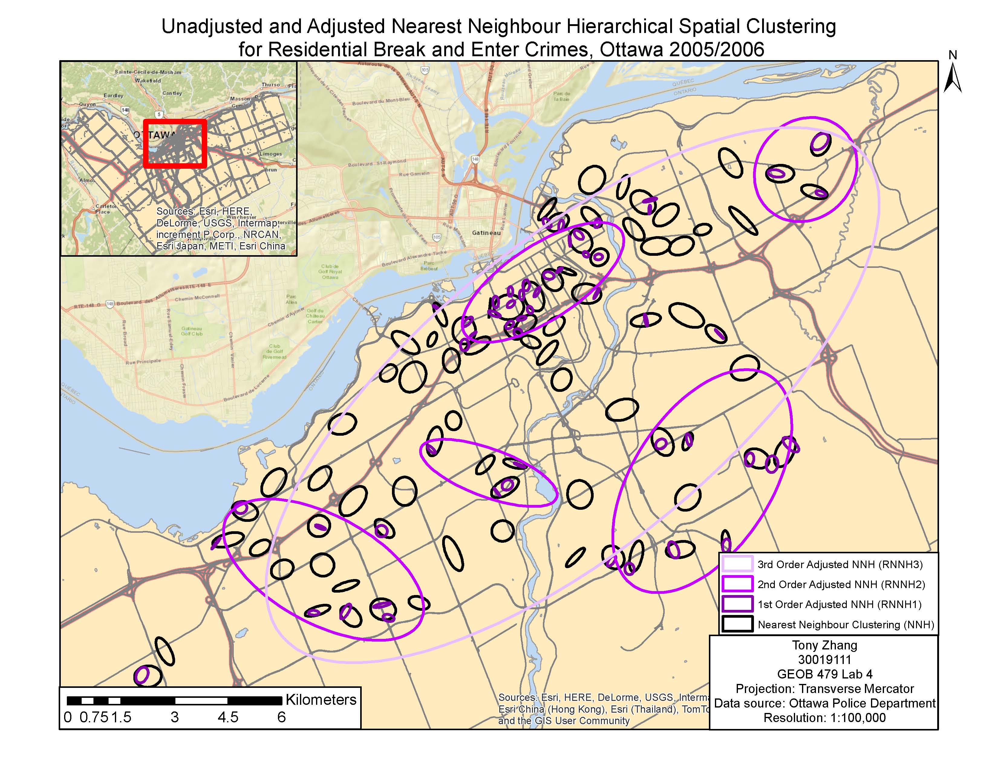
Unadjusted and Adjusted Nearest Neighbour Hierarchical Spatial Clustering