Everything in this model was created using ArcGis Pro software.
Data Collection + Organization
The first step of making this model is to collect the data layers from their sources. These sources can be found in the References page. This specific model only shows the results for the southern half of British Columbia, but all the initial data layers represent all of British Columbia. I set my map processing extent to a polygon of southern British Columbia and my projection-based coordinate system is NAD 83 BC Albers Environmental projection. I made sure to transform any data layers into this projection system, this can easily be done by setting the map projection to BC Albers, so any new data will automatically be transformed to this projection system.
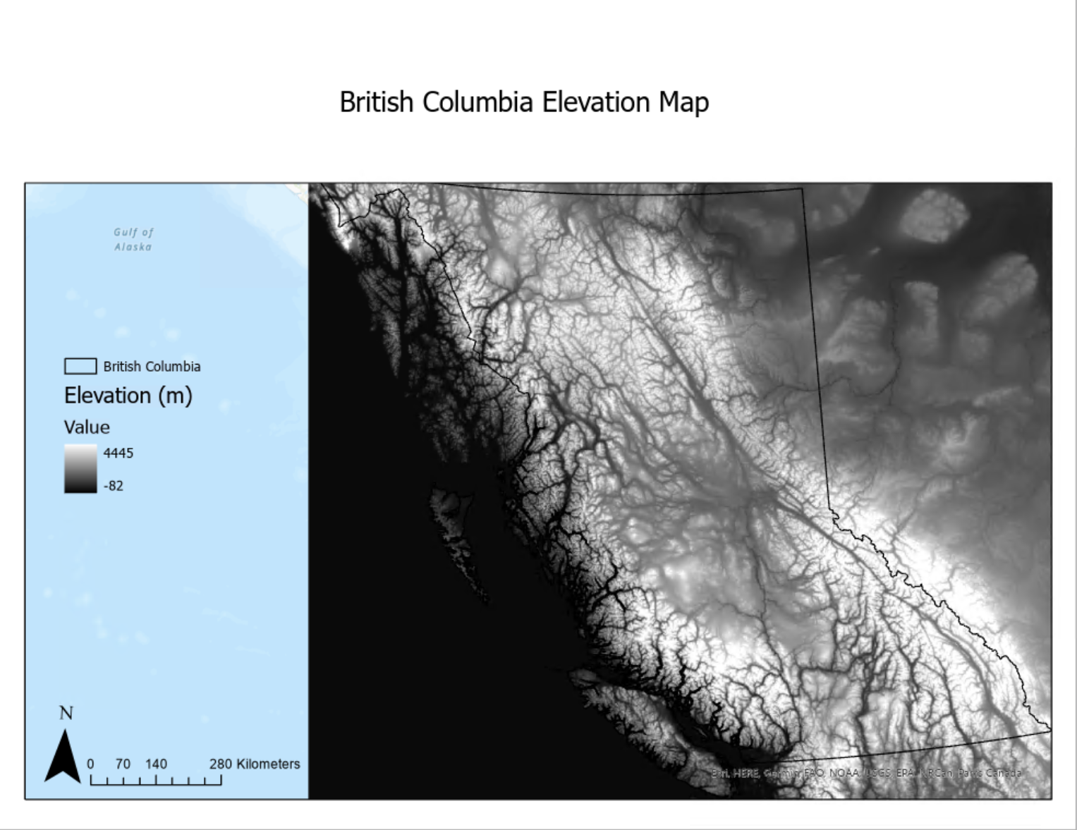
To collect the DEM layer, I plotted rough coordinates of British Columbia into the EarthExplorer program, it does not need to be the exact shape of British Columbia shown in Figure 1 below.

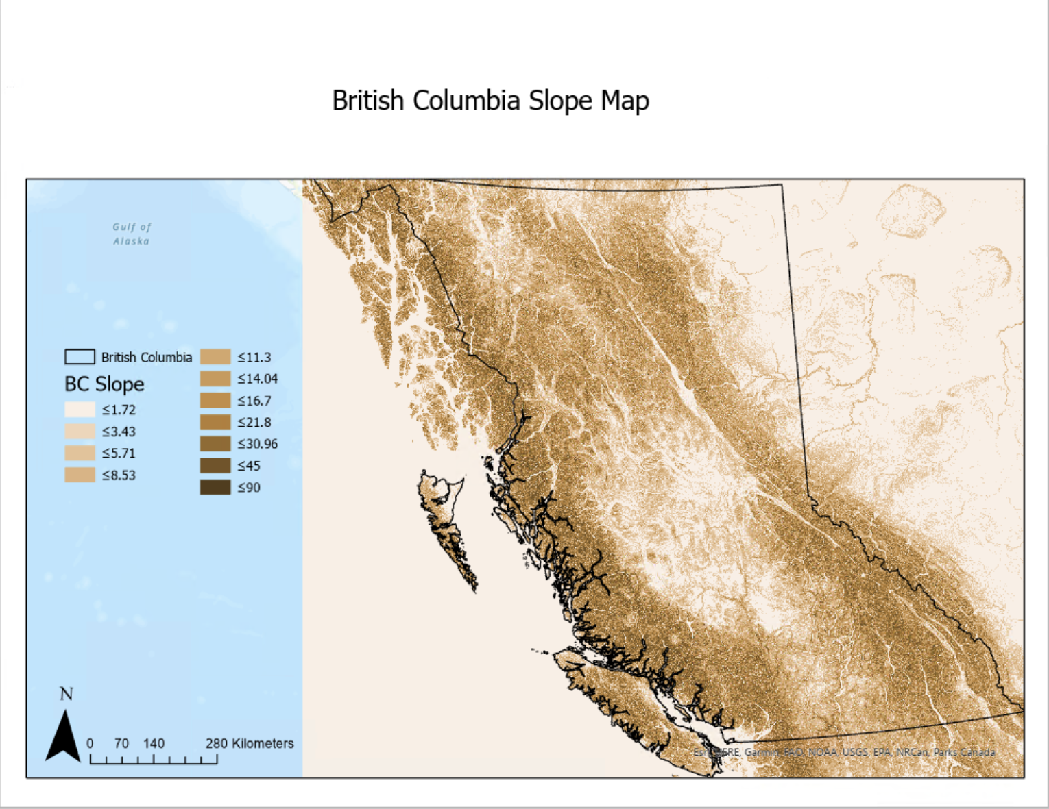
Then, using the slope and aspect geoprocessing tools, I extracted the slope and aspect data layers of British Columbia shown in Figures 2 and 3 below.


Then, creating a new feature class in the catalog pane, I traced the lines of the BC polygon layer to create the BC coast line layer, which was used to calculate Coast Distance. To do this I used the euclidean distance spatial analyst tool. Coast Distance can be seen in Figure 4 below.

There is no need to reclassify these 4 data layers (Figures 1, 2, 3 and 4) as they are all going to stay consistent throughout the temporal study of suitability and can be transformed with the Suitability modeller.
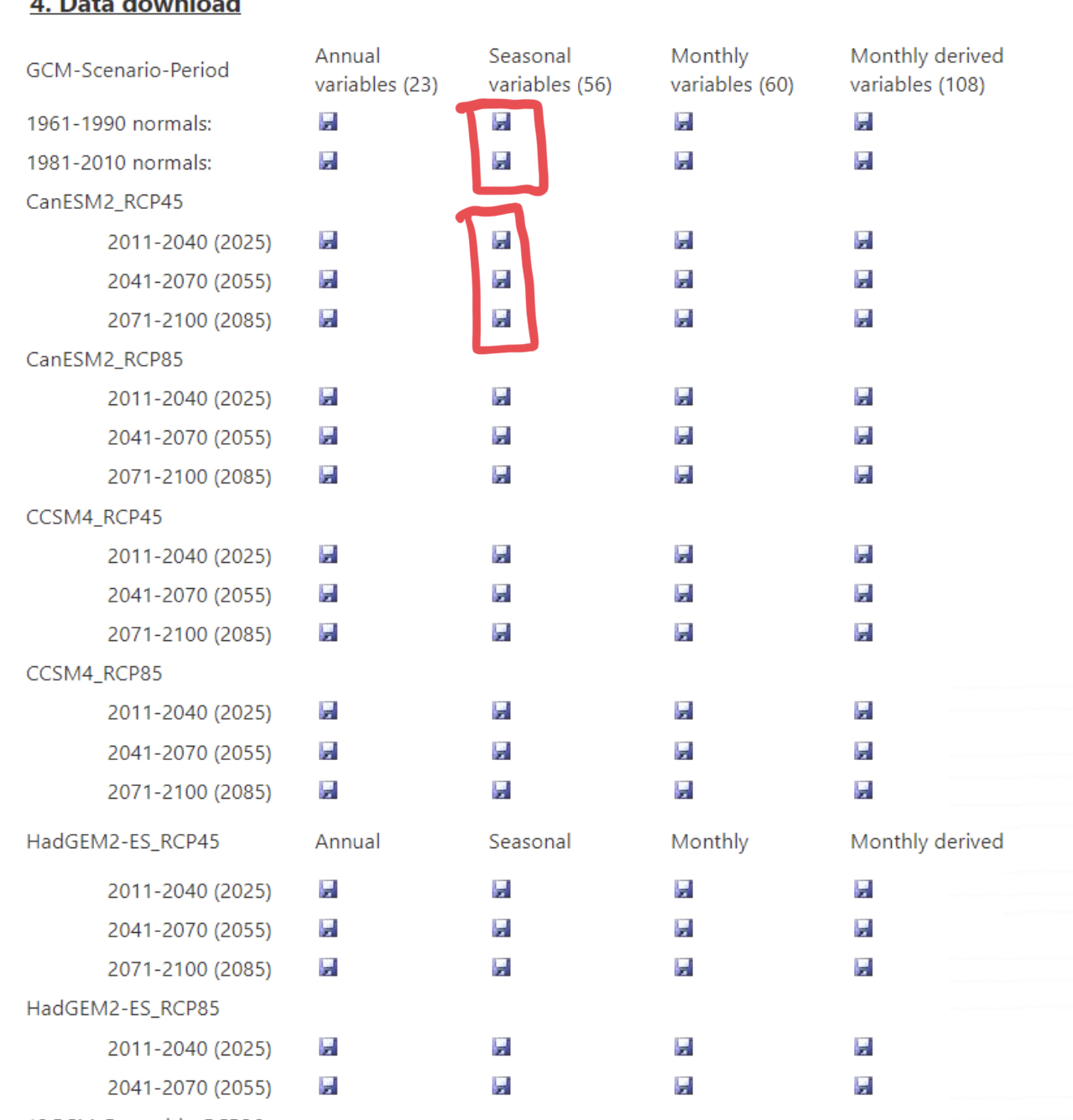
Then I needed to access the ClimateBC raster dataset and download the circled data in Figure 5 below.

Each ZIP file contains 56 different seasonal variables, the two relevant seasonal variables to this study are PAS_wt (winter precipitation as snow mm) and Tave_sm (summer mean temperature C). Then, I needed to delete all the other variables and make sure to label each layer according to the year. These layers don’t need to be reclassified either because the suitability modeller can reclassify and transform the data, standardizing it temporally.
Analytical Hierarchy Process (AHP) Weighting
An AHP generator was used to determine the proper weights for each variable and than a sensitivity analysis for one of the normal periods (1961-1990) was conducted against equal weights.
| Factor | Weight |
| Summer Mean Temp | 31.80 |
| Winter Precipitation as Snow | 31.80 |
| Elevation | 16.50 |
| Slope | 8.50 |
| Coast Distance | 4.70 |
| Aspect | 6.70 |
Suitability Modeller
Five separate suitability models were created for each 30-year normal period, designated from the past to the future, A to E. For the A (1961-1990) model the transformations can be seen below:
| Data Layer | Transformation | Notes |
| Elevation | Continuous Transformation: Inverse Mssmall | <0 = 0 suitability
Anything below sea-level has no suitability for Glacier Growth |
| Coast Distance | Continuous Transformation: Mssmall | |
| Slope | Continuous Transformation: Mssmall | |
| Aspect | Continuous Transformation: Inverse Gaussian | This places highest suitability for north facing slopes, and lowest suitability for south facing slopes |
| Summer Mean Temp | Continuous Transformation: Inverse Linear | >200 = 0 suitability
<0 = 100 suitability If the temp is higher than 20C, max melting can be assumed If the temp is lower than 0C than there is no melting, therefore max suitability |
| Winter Precipitation as Snow | Continuous Transformation: Linear | >2000mm = 100 Suitability
If the snowfall is higher than 2000 mm, that is significant snowfall and therefore high suitability to glacier growth |
The reason limits are given to Winter Precip, and Summer Temp layers is to standardize them against the other temporal models. For example: if 1961-1990 min temp is -7C, while 2071-2100 min temp is 3C, if no restrictions were in place than a suitability of 100 would be given to both, even though in one the snow isn’t melting, and in the other melting is a possibility. This therefore standardizes each set of temp and precip datasets against each-other, and makes sure not to skew the suitability models and properly show the progression of glacier growth locations overtime.
Then, I used the suitability modeller five times, each using the same Elevation, Slope, Aspect and Coastal Distance layers, while switching the Temp and Precip data layers for the different 30-year normal periods.
Sensitivity Analysis
A sensitivity analysis is used to determine uncertainty/error when using mathematical transformations against data, it is used to determine how the inputs actually affect the results, using two different weights of the same transformation.
My last step was to make a sensitivity analysis. This was done by using the locate tool on the suitability modeller for the AHP weights and Equal weights. Figure 6 shows the flow chart. The reclassify tool in Figure 6 converts all values/locations to “1”, so that when the two models are added (the plus tool) the locations which overlap are labelled as 2, while the separate values are labelled as 1.
