Lab 4

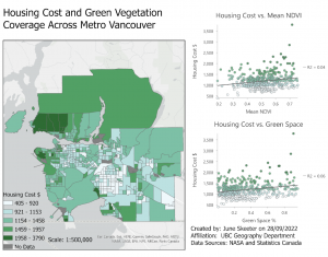
1. NDVI is a metric for gauging vegetation health based on the differential reflectivity of healthy venation (more NIR, less red).  It can be used to identify/distinguish vegetation areas and track vegetation over time.  Values range from -1 to + 1, low values represent non-vegetated surfaces (water, concrete, ice, etc.) + clouds.  High values represent healthy green vegetation. Vancouver – high values in parks (pacific spirit, Stanley park etc.) medium values in single family residential areas, low values over water + downtown/industrial areas.
2. 2.17
3. 0.35
4. 5,045.5
5. DAs have a stronger relationship than CTs, however, neither has a particularly strong relationship as R2 values <0.5 are generally considered weak. You calculated the regression equation Y = mX+b, where Y = “housing” and X = “income” for both the DA and CT layer.  After excluding the zero values: the R2 value for DAs was 0.35, indicating a “weak” relationship, while the R2 value for CTs was 0.23, indicating a “very weak” relationship.
6.  0.6069 
7. The natural breaks classification did a good job of distinguishing areas of green vegetation from urban/water areas. There are always some places where it might be off because of roads or areas with trees that stand alone but overall the natural breaks classification method did a good job. Downtown Vancouver was the area that is the most urban and the model did a good job distinguishing it from less urban places with more tree canopy. 
8. 0.815 
9. 62,777
10. 0.334
11. There is a confounding factor which means the CTs are in different sizes. We have to normalize our data by dividing the sum of the green veg area by the shape area to find out the normalized data. Normalizing is the process where you divide one variable by another to account for their relationship. This can help us find patterns that are masked by the confounding factor. 
12. The are highly correlated (0.83), because they are related to each other, but they do not show the same thing.  Green veg area is a threshold based value to identify the greenest areas as distinct units.  Not all CTs have any “green veg area” at all, when green veg area is low the relationship with Mean_NDVI breaks down, this does not mean they have “no trees”, just that they don’t have any pixels with dense enough concentration, relative to buildings, asphalt, water, etc to be counted.  Mean_NDVI I can tell us the “relative presence of any vegetation”, while PCT_Green_Space is intended to tell us if there are large, continuous patches of present and what proportion of the CTs area they make up.
13. No strong relationships (R2<.1). There are multiple factors that will influence housing cost more directly, for instance housing supply, income, population total, population density, proximity to transit, etc.  OLS lets us account for multiple factors to find a relationship.  Perhaps % greenspace is important, but only once we account for population density and proximity to a transit hub for instance. Two other possible improvements. Also, maybe exclude downtown and just look at single family homes – downtown is a desirable, expensive location where high income people live, but by definition a downtown area will have less green veg. Additionally, could look at proximity to green veg rather than just whether a CT contains green veg.  As is, if the trees aren’t in the CT, the model doesn’t account for it.  But what if a dense CT is next to a large park?  ie. the west end & Stanley park.  – lots of improvements to be made.
14.