
(derived from week 10 lecture material)
Environmental criminology is a sub-division of criminology which focuses on criminal patterns within particular environment and analyzes the impacts of external variables on people’s cognitive behavior. It suggests that crime is a geographic phenomena rather than random process, thus crime mapping and spatial pattern analysis have the potential to help reduce crime. Three central theories of environmental criminology include:
Routine Activities Theory – it is based on that activities of people undertaken on a routine basis (e.g., leave for work in the morning, lock up the store at night…). It predicts that residential homes are burglarized during weekdays in daytime while commercial properties are burglarized during weekend and nighttime. Routine activities not only affect the time of criminal events, and it is obvious that routine activities are not random across space as residential and commercial areas are not randomly located.
Rational Choice Theory – it suggests most offenders make rational decision to commit an offence. This could provide some clues about what an offender is thinking when they decide to commit the crime.
Crime Pattern Theory – it suggests that offenders are influenced by the routines of their lives. They tend to concentrate in areas that are known to them and commit crimes at places without guardians. This can be used to predict where and when the offence would occur.
This three theories reaffirm that crimes are human phenomena, and their distributions are not random across space. Therefore, crime mapping and spatial analysis (e.g., geographic profiling, Centrifuge, CrimeStat) using GIS has became an important practice at most police departments.
Application Example (Lab 4)
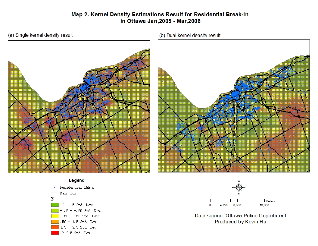
In this example, we will map the spatial distribution of various crimes that occurred in Ottawa between January 2005 and March 2006, and perform spatial statistics using CrimeStat. Crime data in shapefile form were downloaded from the Ottawa Police Department, and used as input to CrimeStat. Nearest neighbour, spatial-temporal hotspot and kernel density estimation analyses were perform in CrimeStat, and then displayed in ArcMap. The nearest neighbour and kernel density analyses were performed twice, with and without the use of a reference file that contain population information. The maps indicate that the crime distribution exhibit clustering at certain areas, and the use of the population reference file made significant impact on the statistic results.
Sample Research Paper Review (Assignment 3)
[Zhang, H., & Peterson, M. P. (2007). A Spatial Analysis of Neighborhood Crime in Omaha, Nebraska Using Alternative Measures of Crime Rates. Internet Journal of Criminology.]
This paper focused on the comparison between three types of measures of crime rates. The three types are: 1. The official measurement of the frequency of crime (official crime rate) defined as the number of incidents of each type of crime committed in an area (e.g., a neighborhood/city/nation…) standardized by the area’s population; 2. Location quotients of crimes (LQCs) which is a ratio between number of incidents of each type of crime in a small area (e.g., a neighborhood) and the total count of each type of crime in a larger reference area (e.g., a city); 3. Crime density – the number of incidents of each type of crime per unit area (e.g., km2) in a given area.
A literature review was conducted by the author, and the major critique found against the official crime rate is the meaninglessness of standardizing by population, because neither criminals nor victims in many cases were from the same neighborhood where the crimes were committed. This is especially common in commercial and tourist zones. In residential areas dominated by apartment complexes, the official crime rate tends to underestimate the risk of crimes as the intensity of crime is diluted by the large population in these areas. On the other hand, LQCs and crime density are not population biased, and the author believes they are superior than the official crime rate in measuring the risk of crimes.
To further compared the differences between LQCs and crime density, hot spot maps for assault, robbery, auto theft and burglary crimes in the city of Omaha, Nebraska were produce. With examples on the map, the author demonstrated the major flaw of LQCs that the LQCs values could be either inflated or deflated for neighborhoods with extraordinary low or high frequencies of crimes.
In addition, the study compared the explanatory power of different Ordinary Least Square regression models (for crimes in Omaha, Nebraska) using the three different types of crime rate measures as dependent variable, respectively. The result indicates that the crime density model had the highest R2 value (0.80), while the LQCs model had the least (0.201). Therefore, the author suggests that crime density is the most effective measure among the three.