
The following section describes the manipulations applied to each data layer, as referenced in Figure 1, prior to their input into the MCE model. The data inputted into the model included slope, precipitation, vegetation, bedrock geology, and proximity to fault lines.
Slope
A digital elevation model provided from the ESRI 2010 dataset was manipulated to calculate slope. Using the Spatial Analyst Tool > Surface > Slope operation, we were able to create usable data for this factor in our weighted analysis. High slope values indicated high landslide susceptibility areas, and are indicated by red in Figure 2. Areas of green suggest low slope values.
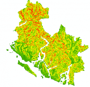
Figure 2: Raw slope data of region
Precipitation
As slope stability can be heavily influenced by soil saturation, precipitation data was used within our MCE model to determine areas that may experience higher soil saturation throughout the year. No further manipulation to the clipped and projected precipitation dataset was required at this point. Areas of Figure 3 in blue indicate the lowest precipitation within this region, whereas red indicates areas of high precipitation.
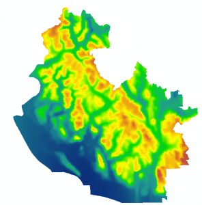
Figure 3: Raw precipitation data of region
Vegetation
Plant cover provides soil cohesion and reduces rainfall impact on soil, which contributes positively to slope stability (Wu & Chen, 2009). Our downloaded data was collected via remote sensing and classified using a normalized difference vegetation index (“NDVI”). Two potential sources of error presented within this dataset were associated with some regional areas missing data, and some data being classified as cloud shadow.
Areas missing data were observed generally in high altitude regions associated with heavy snowfall and high slopes. It was assumed that these areas did not reflect wavelengths within the photosynthetically active radiation spectral region due to lack of vegetation or heavy snow cover (Gates, 1980). Therefore, we assumed these regions were located above the tree line in a zero vegetation cover zone. These no data regions were incorporated into a new polygon layer by selecting areas that contained vegetation areas, and using the Erase tool to remove them from the layer. This layer was then merged with the vegetation layer and attribute table using the Union tool to create a new vegetation layer that included data in these no vegetation zones.
Cloud shadow areas represented areas within the remote sensing data where clouds or cloud shadow caused data collection interference. Because the data within these areas were completely unknown, we considered them to be high landslide susceptibility regions to remain conservative in our results.
Vegetation data was then reclassified into generalized categories and assigned friction values between 0 and 1 and ranked based on canopy density (Table 2) in order to input the data into the MCE model. A low ranking refers to inferred stronger root cohesion and slope stability, and therefore would correlate with a decreased susceptibility to landslide occurrence A value of 0 refers to dense vegetation (high slope stability), and a value of 1 refers to areas of no vegetation that would be indicative of low slope stability.
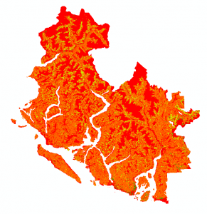
Figure 4: Raw vegetation data of region in polygon format
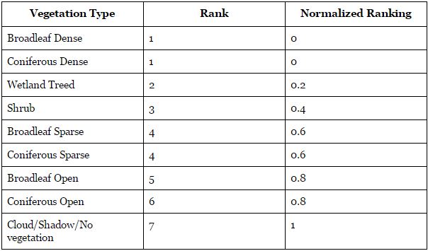
Table 2. Normalized ranking of vegetation type.
This data was then converted from a polygon to a raster with cell sizes of 100 X 100 m.
Bedrock Geology
Similar to vegetation types, bedrock geology was categorized and ranked based on the strength of each rock type identified within the region of interest. Stronger rock was associated with stronger slope stability, and therefore a lower susceptibility to landslides. The strength of each rock type was determined previous knowledge on rock type properties, and from the website Compare Rocks.
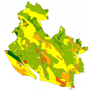
Figure 5: Raw data of region in polygon format
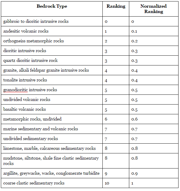
Table 3: Normalized ranking of bedrock geology in region
After reclassifying each rock type, the polygon layer was then converted into a raster layer with a cell size of 100 x 100 m.
Proximity to Fault Lines
Fault line data has been used in multiple studies when modelling landslide susceptibility (Shahabi & Hashim, 2015; Wu & Chen, 2009; Komac, M. (2006)), and was incorporated into our MCE model by determining an area’s proximity to existing fault lines. In addition to the importance that fault line proximity had played in other academic literature regarding the subject of landslides, proximity to fault lines was taken to account due to the high seismic activity that is expected to occur in British Columbia.
The Spatial Analyst Tool > Proximity > Euclidean Distance tool was used to identify a continuous region of decreasing landslide susceptibility surrounding fault lines. Areas closest to the fault lines represent a higher risk of landslide occurrence. Distant region represented areas with lower landslide susceptibility based on potential seismic activity. Red areas within Figure 6 indicate a close proximity to fault lines, where as green areas represent further distance.
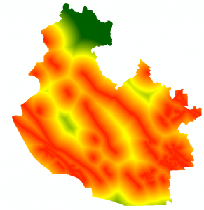
Figure 6: Euclidean distance from fault lines in region