Author Archives: Lucia Marie Bawagan

UBC BSc Geographical Biogeosciences

Investigating the Impacts of Spring versus Winter Lake Eyre Dust Storms

Applications of Online Trajectory and Dispersion Models

Objectives: Explore the application and limitations of air quality models while investigating the role of synoptic situations on plume dispersion.

  • Assume a potentially large explosive point source in a chosen location, with a major release of pollutants. Examine and describe the transport of material pollutants over 72 hours after the 6 hour release of materials using the HYSPLIT online trajectory model.
  • Plot synoptic maps for the chosen period of time of the given release of pollutants from an online map plotting archive. Investigate the possibility of precipitation and cloud interference using archived satellite imagery.
  • Assuming the data used is forecast data, provide advice on the nature of impacts and the affected regions over the 72 hour period by comparing two different dates of potential pollutant release and illustrating how differences in synoptic situation produce different impacts.

Abstract

Online trajectory and dispersion models were used to estimate and compare the behaviour of spring and winter dust storm pathways from the Australian Lake Eyre basin. Based on a 2009 spring dust storm, the Hysplit method approximated the spatial extent and persistence of Lake Eyre dust transport within the northeast coast of Australia, and cross Pacific to Indonesia and New Zealand. This was compared to winter dust storm conditions projected for June 23, 2009. The spatial and temporal extent of these dust pathways suggest significant local and international, environmental and human health impacts. Although, it should also be noted that these models of study are limited by restrained time parameters and lacking information on temperature, humidity, and complex terrain effects.

See full report here: LakeEyreDustStorm_FinalReport


Source Links & Statements

Barlow, K. (2009, September 25). Dust storm chokes Sydney. ABC News. Retrieved from www.abc.net.au/news/2009-09-23/dust-storm-chokes-sydney/1438510

McGowan, H.A., McTainsh, G.H., Zawar-Reza, P., Sturman, A.P. (2000). Identifying regional dust pathways: application of kinematic trajectory modelling to a trans-Tasman case. 26:5, 633-647. Retrieved from http://onlinelibrary.wiley.com/doi/10.1002/1096-9837(200006)25:6%3C633::AID-ESP102%3E3.0.CO;2-J/full

McGowan, H.A., Clark, A. (2008). Identification of dust transport pathways from Lake Eyre, Australia using Hysplit. Atmospheric Environment. 42:29, 6915-6925. Retrieved from https://www.sciencedirect.com/science/article/pii/S1352231008004950?_rdoc=1&_fmt=high&_origin=gateway&_docanchor=&md5=b8429449ccfc9c30159a5f9aeaa92ffb

McKendry, I. (2018). Hemispheric scale transport processes [PDF document] Retrieved from http://ibis.geog.ubc.ca/courses/geob402/lecture.html

Safe Driving Routes in the Greater Vancouver Regional District

Objective. Determine the safest driving routes from the UBC Vancouver campus to randomly selected neighborhood points within each of the following cities in the Greater Vancouver Regional District according to a cost surface: Vancouver, Richmond, Burnaby, and Surrey. Design a cost surface based on the spatial distribution of car accidents that occurred in 2015 and perform a Kernel density analysis to determine the relative concentration of car crash counts and car crash types.

See full report here https://blogs.ubc.ca/drivingroutesubc370/


Regression & Correlation Analysis of Crime in the City

Objective. Explain and analyze the concept of spatial autocorrelation regarding median total household income and the occurrence of different types of crime in an urban setting. Explain and show evidence of the ways in which the Modifiable Areal Unit Problem (MAUP) impacts analyses via the scale and aggregation effects, as well as the implications that these uncertainties might represent when interpreting the results of the spatial analyses. Manipulate and analyze census data and work with statistics tools for spatial data.

Statistics Canada: Data Suppression in Dissemination Areas.

There need to be more than forty people living in a dissemination (enumeration) area to keep Statistics Canada from supressing census characteristic data for that geographic area. For income data, there need to be more than two hundred fifty people to keep Statistics Canada from practicing area suppression.

Statistics Canada practices area suppression to protect the privacy of individual participants in the given statistical study.

Random rounding is an area suppression technique where values “greater than ten are randomly rounded up or down to multiple of five [and those less than ten] are randomly rounded to zero or ten” (Puderer, 2001). This decreases data precision by normalizing the data into random multiples of zero, five, and ten, which will affect the implications drawn from generalized data values.

Spatial Autocorrelation of Residuals.

The residuals are spatially auto correlated. This is supported by the Moran’s Index report which shows that the spatial distribution of crime is clustered, and not randomly dispersed for both maps: also indicated by the z-scores and p-values shown in Table 1.

Regarding the distribution of residential break and enter crimes, the results of the residual analysis show whether the predicted value of crime incident in a neighborhood is greater than, less than, or approximately equal to the observed number of neighborhood crimes. As shown in the map, “Regression Analysis of Vancouver Residential Break and Enter Crimes and Median Total Household Income Correlation Model,” the neighborhoods coloured closer to the dark red shade are associated with observed crime greater than the predicted value and those closer to the dark blue shade are associated with observed crime less than the predicted value. The neighborhoods colored in pale yellow are those with observed crime values closest to the predicted value: where the relative abundance of these areas support that the residuals are spatially auto correlated.

See Regression Analysis of Vancouver Break and Enter Crimes and Median Total Household Income Correlation Model

Residual Patterns in Census Tracts and Dissemination Areas.

Dissemination areas are census data measured in smaller geographic units compared to census tracts maps. So the residuals represent similar patterns in both maps but the census tracts map shows a more general distribution of residential break and enter crimes: class breaks are larger areas assigned with the same colour. These groups are subdivided into smaller areas with varying colours in the dissemination areas map. The dissemination areas show different crime intensities concentrated in smaller tiles within the same census tract.

The census tracts map shows the largest deviation from the average frequency of break and enter crimes generally occurs within the same areas, but the dissemination areas map shows that they are concentrated into smaller areas. Regarding medina total household income, greater deviations (whether greater or less than) from the mean represent the degree of auto correlation between median total household income and crimes. The patterns show whether our function for crime and median total household income predicts well or poorly.

The scale affects the map user’s understanding of the distribution of residential break and enter crimes relative to median total household income. The data is averaged across a larger area in census tracts than in dissemination areas, so changing the scale will also change the distribution of the data per census tile (distribution of different colours per census tile in the map). It can imply a more clustered versus dispersed distribution of the correlation.

See Regression Analysis of Vancouver Break and Enter Crimes and Median Total Household Income Correlation Model

For example, the 0049.01 census tile has a 0.5-1.5 standard deviation in the census tracts but the dissemination area shows that approximately 60% of that census tile has a concentrated standard deviation greater than 2.5

In the 0057.02 census tile, the census tracts map shows a standard deviation greater than 2.5 but the dissemination areas show this standard deviation value concentrated only on approximately 15% of that census tile.

Grouping Analysis for Census Tracts and Dissemination Areas.

The groups are labelled according to the relative variation of neighborhood crime according to median total household income. Income and crime are ranked separately as values greater than, less than, or average compared to other neighborhoods, and the variance of income and crime levels are approximately equal for both maps.

The two maps both show the occurrence of neighborhood crimes related to median total household income: neighborhood crimes considering only mischief, auto theft, and residential breaking and entering. They show that neighborhood crimes tend to occur in low to average (medium) income neighborhoods.

In general, the results of the grouping analysis do not support the claim that income and security in Vancouver are related Despite there being a potential positive relationship between median household income and neighborhood crime, as suggested by the residual analysis, the grouping analysis suggests that this might not be the case. Other than relatively high crime rates occurring in low to average income neighborhoods, the grouping analysis suggests that there could be other variable not accounted for in the analysis but may still affect the distribution of neighborhood crimes. Although it is possible that higher income neighborhoods provide a greater incentive for residential breaking and entering, other factors such as a neighborhood’s proximity to crime hot spots, could affect the actual spatial distribution of crime in Vancouver.

See Grouping Analysis of Vancouver Neighborhood Security in Relation to Median Total Household Income

See full report here Correlation and Regression Lab Report
Testing for Variance in Mean Annual Storm Water Discharge

A geostatistics report for Testing Variance in mean annual storm water discharge for the Assiniboine River At Headingley, Winnipeg

Objective. Use ANOVA to test for variance in the mean discharges per June day from 2007 to 2016, measured at a single hydrometric station, to determine whether to support or reject the null hypothesis.

Null hypothesis. There is no significant difference between mean annual discharge for each June day in the past decade: implying a change in the methods of storm water management as a non-necessity for the locality.

Alternative hypothesis. At least one June day has a mean discharge that differs significantly from other years in the past decade: implying a change in storm water management as a necessity and potentially warrants the Calrossie-Cockburn project.

SEE FULL GEOSTATISTICS REPORT HERE: TestingforVarianceinMeanAnnualStormWaterDischarge_FinalReport

Source Links & Statements.

Bodnaruk, B., Curi, F., Ewing, J., Houston, R., Huth, A.K., MacMillan, D., Parente, M., Sharp E., Turcotte, D., Volden, R., Wilcox, M, Zhu, J. (May 2010). Cockburn and calrossie combined sewer relief works project final conceptual report. Retrieved from http://winnipeg.ca/waterandwaste/drainageFlooding/pdfs/CockburnCalrossieFinalReport_web.pdf


Water Survey of Canada – WSC. (191-). Historical hydrometric data [Data file]. Available from https://wateroffice.ec.gc.ca/google_map/google_map_e.html?map_type=historical&search_type=province&province=BC


Winnipeg Water and Waste Department – WWWD. (April 10, 2017). Cockburn and calrossie combined sewer relief works project. Retrieved from http://winnipeg.ca/waterandwaste/drainageFlooding/cockburn_calrossie_cso.stm

Digital Terrain Modeling & Multi-Criteria Evaluation (MCE) Analysis – Determining Potential Habitats for Spiranthes diluvialis in Southern Okanagan

Objective: Produce a multi-criteria model to assist in directing the search for potential habitats for the species, Spiranthes diluvialis, given a set of predetermined criteria for their preferred living environment: namely, low-slope, mid-elevation areas with a southern aspect approximately 725 hectares worth of total potential space. Construct digital terrain models (TINs, DEMs) to aid in constructing a geographic information surface to conduct the above MCE analysis.

“The Triangulated Irregular Network (TIN) model recreates a topographic surface by connecting measurable points of elevation with lines of slope and planes of aspect. A Digital Elevation Model (DEM) uses a raster, or cell-based, approach to represent topography” (UBC Geography, 2017).

Using Contours in GIS Analyses

Contours are not typically used in GIS analyses because they are not spatially continuous and therefore, can not easily interpolate the data: whereas GIS analyses rely on continuous iso-lines. For features like the unclosed lakes previously represented as line data, such would need to be converted into closed polygons by manual edge-matching. However, edge-matching assumes that the missing edge of the feature is perfectly straight and would thus decrease the accuracy of the feature representation.

Defining XY Tolerance

The XY Tolerance tool is used to group features with similar geometry, wherein the set XY tolerance value used is the shortest distance in between two clustered coordinate features: or rather, the minimum resolution of joining feature points to make lines and connecting line segments to create closed polygons. In this case, the XY tolerance (two meters) was used to connect line segments to create closed polygons in order to represent the lake features.

Setting too large an XY tolerance will over generalize the data by combining nearby lakes and showing them as one polygon. Setting it too small might not connect enough of the line segments to create a closed polygon of the lakes.

Digital Terrain Modeling Manipulation See attached map, ‘TIN Analysis of Southern Okanagan” for practice on digital terrain modeling manipulation.

TIN Analysis of Southern Okanagan

Selecting midpoints in Defining Areas with Southern Aspect

Selecting 180° (instead of 45°) as the midpoint assures that any aspect close to 180° degrees will have a southern aspect. When starting the degree measurement at 0° North, the convention is clockwise from North of the degree arc, such that 180° will always be perfectly South. Choosing 45° as the midpoint would define areas with a North eastern aspect.

Procedure

It was given that the preferred living conditions of the Spiranthes diluvialis, the area of interest would be approximately 725 hectares of low slope, mid elevation area with a southern aspect. The provided  elevation, water, and transportation shape files were converted into feature classes to construct a TIN, and later a DEM, to be examined using a multi-criteria evaluation (MCE) model by the following procedures: factor identification, data normalization, and multi-criteria analysis. The ideal habitat factors, namely low slopes, mid elevation, and southern aspect, were normalized by establishing an ideal value within a range of reclassified values. Elevation was normalized around an ideal 750 meters, slopes around ‘low’ and aspect around 180° south. Values close to the ideal parameters were reclassified values close to 1 and otherwise, reclassified values closer to 0. The normalized data was tested by weighted importance in 2 MCE models to examine the spatial variability of assigning equal versus unequal weighted importance shown in the attached map, “Potential Habitats for Spiranthes diluvialis in Southern Okanagan.” weighted importance for the MCE models was calculated using the analytical hierarchal approach (AHP) calculator: see Fig. 1 and Table 1 below.

Figure 1. Equally and unequally weighted importance comparison using AHP calculator

Equally and Unequally Weighted Comparison Figure


Table 1. Equally and unequally weighted importance comparison using AHP calculator

Equally and Unequally Weighted Comparison Table


Multi-Criteria Evaluation Results

The first MCE model assumes equally weighted importance, assigning each factor 33% of importance. The map, “Potential Habitats for Spiranthes diluvialis in Southern Okanagan,” shows that 474 cells are potentially ideal habitats. The second MCE model shows an unequal weighted comparison wherein aspect (50%) is weighted greater than slope (25%) and elevation (25%), yielding 149 cells of potentially habitable area. This comparatively more restrictive weighted comparison would be helpful in cases when alternative habitats would need to be considered. The weighted sum for the MCE shows areas of overlap between infinite combinations of varying equally and unequally weighted comparisons: 2, 051 cells. This is important in considering how the spatial variability of potential habitats changes when varying the weighted importance. The suggested survey area is the overlapping region of the equally and unequally weighed importance, totaling 623 cells.

See attached map, “Potential Habitats for Spiranthes diluvialis in Southern Okanagan”

Potential Habitats of Spiranthes diluvialis in Southern Okanagan


Least Cost Path Analysis – Transmission Station to Manufacturing Plant Route

Objective: Determine the least cost path of a feeder line running from transmission station to manufacturing plant over a predefined cost surface, and compare this to the shortest path route

The concept of a ‘cost distance’ is typically used to model movement through space where frictional elements that might impede movement are defined. Here, the cost of having a feeder line run between the source and destination feature is studied according to the different frictional values assigned to areas based on their land use. See attached map, “Transmission to Manufacturing Plant Route: Shortest versus Least Cost Path.”

Transmission to Manufacturing Plant Route: Shortest versus Least Cost Path

The length of the shortest path route was calculated by summing the attribute ‘value’ and ‘count’ products from the extracted land data layer. It was found to be approximately 38, 925 meters long with a total frictional cost of 1, 871, 875 units. The length of the least cost path is found directly on the attribute table of the associated data layer and is approximately 50, 354 meters with a total frictional cost of 281, 255.10 units.

Distinguishing between the least cost path and the shortest path route

Least Cost Path: The land area surrounding the start (source feature) and end point (destination feature) of the manufacturer’s feeder line are assigned friction values that indicate the ‘cost’ of passing by areas based on their land use. So the least cost route should pass by open areas and resource and industrial areas that are base cost, and try to avoid passing high cost areas like residential neighborhoods and water bodies. After creating a matrix that ranks the spatial variability of cost via land use, the least cost path route is drawn along a path that avoids high cost areas. This makes the route dependent on the assigned friction values of passing high versus low cost areas: wherein cost defines the monetary/economic, social, political, and environmental drawbacks of constructing the feeder line along certain areas.

Shortest (Euclidean Distance) Path: The shortest path route is generally a straight line path that runs from some starting point (the transmission station) to some end point (the manufacturing plant) and does not consider the social implications of friction cist. For example, it does not take into account the hindrance that a feeder line would cause in population dense areas nor the environmental complications in vegetation and fauna population dense areas.

Representation of Water Features in the Least Cost Path Route: Data for water features need to be converted from vector to raster data on the map after edge matching lakes to form closed polygons for the analysis. The raster map reduces the representation by opting out streams and thereby allowing the least cost path of the prospective feeder line to cross these streams. This problem mainly concerns how grids representing rivers allow crossing and so we can convert the domain shape of resolution from a square grid to a hexagonal grid when converting from the vector to raster representation of the data. The six sides of each hexagon on the grid will disallow crossing by closing gaps between each repeated polygon.

Routing over Existing Transmission Lines and Highways: For the least cost path to avoid routing over highways, assign medium to high frictional values to major roads and highways by adding another column in the attribute table of the associated data layer: named ‘cost.’ Input some frictional value greater than residential and commercial areas or some friction value less than or equal to those of water bodies.

Ideal Living for Senior Citizens in Vancouver

Final Project: Analysis of ideal living areas for the Vancouver elderly population according to select areas’ accessibility to needed and preferred public service facilities; areas found using ArcGIS and data from Vancouver data catalogue.


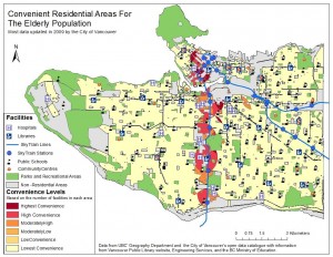
Our goal for this project was to find areas within Vancouver that would be considered ideal living for the local elderly population that are either financially or physically unable to use mobile vehicles. We defined these “convenience areas” as those accessible to general public service facilities, and therefore by their proximity to these facilities. Our GIS analysis would then find these convenience areas within the buffer zones of all facilities. To depict a range of convenience areas, we defined those of “highest convenience” to be those areas within the proximity of all facilities whereas “low convenience” areas were those within the proximity of just (any) one of the select facilities.

Seeing as this project assumes a general audience (i.e. the elderly), our definition of convenience areas is subjective and can thus seem too narrow of a criteria to define the needs and preferences of the elderly regarding their ideal living space. Although this was also part of our original goal, it was understood that more data was needed to provide a more in depth analysis on the matter. As mentioned in the report linked below, data on the needs and preferences of senior living homes, as well as the current and projected financial capabilities and options of the elderly population would benefit further analysis on this topic.

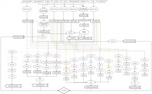
Our method of analysis required multiple steps, as described on the project report below, such that all group members had to work on the map together as opposed to dividing the tasks and working on parts of the map separately.

Project Report attached gives a description of the project, the study area, the methods of our group analysis, results, and a discussion on further research that could improve our method of finding areas that would be ideal living for a range of physically able senior citizens in Vancouver.

Attached below is a flowchart that outlines the procedures of our analysis for finding these ideal living areas through ArcGIS.

Flowchart

Attached below is a map of the areas that we would recommend for senior citizens to live in Vancouver. As described in the report linked above, we define areas of convenience to be those within an 800 to 1000 meter radial proximity of select public service facilities such as parks, community centers, libraries, schools, transit stations, and hospitals.

Map_CRAVP

Accomplishment/s:
Examined ideal living areas for the Vancouver elderly by their accessibility and/or proximity to select public service facilities

Environmental Assessment for Proposed Garibaldi Ski Resort

Lab 5: Assessing the Environmental Risks of a Proposed Development Project


EIA_Garibaldi shows an environmental assessment for a proposal to construct a ski resort in Garibaldi Park, at Squamish.

Hillshade_EIA shows the lighting or shading effect of the sun incident on a landscape of varying elevations, a Hillshade.

EIA_ClientMemo includes a client memo that summarizes the methods and results of my analysis, as well as some recommendations to aid my client in the direction and focus of their project proposal.

Personally, I do not think this project should continue unless they find a way to integrate the construction and operation of the ski resort into the original ecosystem, so as to minimize potential environmental risk. This does not differ from what I wrote in my memo, since it would be in my client’s interest to assuredly maintain economic viability by minimizing their project’s environmental risk. Environmental projects are generally complicated because they challenge personal and group ethics, making it difficult to determine whether overall social, economic, and/or cultural benefits outweigh the environmental costs in both the short and long term. This project, in particular, is problematic as it is subject to some degree of scientific (information deficit) and moral (understanding) uncertainty, and the overall complexity and unpredictable responses of natural versus anthropogenic working ecosystems needs to be considered. Information deficits are elements of the “known unknowns,” that is the information we know we do not have, and “unknown unknowns,” that is the information we do not know we don’t have. Moral certainty and uncertainty is then built on this information or lack thereof. System complexity and unpredictability, on the other hand, is a problem evident in this analysis. The near-half percentage of environmental damage from constructing the ski resort alone poses a significant risk against the project. Interconnectedness of ecosystems make anthropogenic interference with them unpredictable and costly. That and with a local percentage of 48.5% of protected area at risk, it is assumed that the overall percentage of risk from a macro-scale environmental assessment (which would include species and ecosystems outside or just surrounding the project boundary area) would be underestimated. Underestimating risk would then give way to great and unpredictable consequences.


Accomplishment/s:

  • Assessed potential environmental impacts that would impede long term economic feasibility of the proposed project to be insufficient for approval
  • Recommended alternative action plan for an environmentally integrated business establishment for reduced environmental risk and economic sustainability

Tsunami Danger Analysis of Metro Vancouver

Lab 3: Tsunami Risk Assessment of the Metro Vancouver Area


TsunamiRiskAssessment_FinalMap shows a map of danger zones if a tsunami were to hit Vancouver. These danger zones include land areas that lie within 1 km. of the shoreline and at elevations below 15 meters given a tsunami wave 15 meters high: namely, road networks categorized by road type and affected areas categorized by land use. With this, I labeled ideal points where precautionary signage could be placed to warn the public of these danger zones: labeled on the map as ‘signage.’

As categorized by land use, the tsunami danger zones include health and education facilities. The healthcare facilities at risk include False Creek Residence, Broadway Pentecostal Lodge, Coastwest Community Home, Yaletown House Society, and Villa Cathay Care Home. The education facilities at risk include Ecole Rose Des Vents, St. Anthony of Padua, Heritage 3Rs School, Vancouver Montessori School, False Creek Elementary, Henry Hudson Elementary, Emily Carr Institute of Art and Design, St. John International, St Francis Xavier, and the Institute of Indigenous Government. To do this, I used an ‘overlay-intersect’ tool that allows me to create a new map layer that includes the health and education facilities within the boundary of tsunami danger zones: i.e. health and education facilities within 1 km. of the shoreline and at elevations below 15 meters.

Approximately 52% of Vancouver is in danger of a tsunami. To find this, I first used data from a digital elevation matrix (DEM) to highlight areas at elevations below 15 meters and hence, would likely be affected by the tsunami and intersect this data with coastal areas 1 km. away from the shoreline. This gives the total area of tsunami danger zones: 665 km2. Then divide this by the the total area of the area of study (Metro Vancouver).


Accomplishment/s:

  • Investigated qualitative and quantitative tsunami risk through calculations and spatial analysis
  • Outlined tsunami danger zones and points of interest for warning signage as an aid to establish tsunami hazard prevention plans
  • Evaluated potential health and education facilities at risk for improved urban planning


Vancouver-Ottawa Housing Affordability

Lab 4: Comparing Vancouver and Ottawa Housing Affordability according to housing cost and household income


Affordability shows a visual comparison of Vancouver-Ottawa housing affordability using the manual breaks classification method. As opposed to displaying housing cost, which includes price information alone, ‘affordability’ refers to the ability of a single or cumulative income to purchase a house of some cost. This makes it a better indicator of housing affordability than housing cost as it integrates income and cost information. As determined by the 12th Annual Demographia International Housing Affordability Survey 2016 (Wendell Cox Consultancy & Performance Urban Planning: Christchurch, New Zealand), housing affordability rating categories range from a median multiple of under 3.0 being ‘affordable’ to over 5.0 being ‘severely unaffordable.’ This makes ‘affordability’ a potentially good indicator of a city’s ‘livability.’ It is worth noting also, that housing affordability analyses may only give information on single detached housing whereas a city’s livability refers to multiple residential types such as single detached housing, multiplex housing, apartments, condominiums, lane housing, and school housing.

Accomplishment/s:
Analyzed interregional housing affordability according to quantitative survey census tracts

Organized and displayed findings according to differential break classification methods