To answer the research questions, there were three parts of the analysis that were conducted: a regression analysis on housing supply change and housing cost change between 2011 and 2016 to explore the impact of supply on housing cost to briefly explore the ideal “how” of action on housing, a multi-criteria evaluation to explore where action on housing was needed and where it would be considered good land-use planning given proximity to services, and a querying process by which specific single and two-family zoned areas were identified for re-zoning. I will review first how data was acquired and managed, and then how these analyses were conducted.
Data
Spatial data was retrieved from two sources: Statistics Canada and the City of Vancouver Open Data Catalogue. Statistics Canada contained the shapefiles of the dissemination area polygons for Greater Vancouver that could be clipped to the extent of the city of Vancouver, and the Open Data Catalogue contained vector shapefiles for roads, the location of community centres, schools, and rapid transit stations. The rapid transit station shapefile was modified to include additional points to represent the eventual locations of stations along the Millennium Line Broadway Subway extension.
As for attribute data that would be joined to dissemination area polygons, this was retrieved from a combination of University of Toronto’s CHASS Data Centre for the Canadian census, and directly from the Statistics Canada website in the form of an IVT file that had to be dissected in Beyond 20/20 in order to extract attribute data for mode of transport and commute time that was not available in the CHASS Data Centre for 2016. It is important to note that data from the 2011 National Household Survey carries a degree of uncertainty with it because it was voluntary: in Vancouver, this is measured as a 24.4% global non-response rate.
After variables on median household income, median shelter costs, median monthly rental costs, total dwellings, rental dwellings, median commute time, and mode of transport were acquired from the CHASS Data Centre and the Statistics Canada IVT file for both the 2011 National Household Survey and the 2016 Census, I managed them on excel to transform the extensive variables to intensive variables when appropriate, and to derive the differences in values between 2011 and 2016 for income, shelter costs, and number of dwellings that would be necessary for the regression analysis and the multi-criteria evaluation that follow.
Regression Analysis
A simple regression analysis was conducted using the Ordinary Least Squares function under the Spatial Statistics tools in ArcMap with ratio change shelter cost between 2011 and 2016 as a dependent variable to evaluate its relationship with ratio change in number of dwellings between 2011 and 2016. The objective of this was to determine if positive local changes in supply would have a negative effect on shelter costs, and if so, to use the residuals of this model in the following multi-criteria evaluation as a way of avoiding areas in the city where adding supply has not led to increased affordability (e.g. lower or stable shelter costs relative to income).
Multi-Criteria Evaluation and Areal Interpolations
For this section of the methods, I will begin by explaining what criteria I selected for the multi-criteria evaluation, followed by the methods by which I created the necessary raster surfaces to input into the Weighted Sum Spatial Analyst function which yields its results. Below I enumerate the criteria selected in order of importance, followed by the reason why it was used, and its weight out of 1 that was used in the Weighted Sum function on the basis of its relative importance to other criteria:
- Proportion of rental dwellings to total dwellings is the most important criteria because it targets areas of the city where the rental market is prominent and can be expanded to prevent displacement and house additional families and vulnerable populations. Weight: 0.3
- Ratio of median shelter cost / median income primarily highlights parts of the city with single-family houses whose values have risen dramatically in spite of the lack of a rise in household income to match it. While in highlighting mainly parts of the city with high ownership rates – and thus low risks of displacement compared to rental-prominent areas – it highlights parts of the city that have become unreasonably inaccessible that ought to be addressed in some capacity to make space for new residents. Weight: 0.15
- Ratio of median monthly rental costs * 12 / median income is a similar metric to above but underscores the affordability situation for rental housing tenants as opposed to primarily owners. These two metrics are complementary. This is merely a proxy criteria since the median income of renters cannot be known from publicly available census data, so I’ve assumed that it follows patterns similar to total median income. Weight: 0.15
- Rate of sustainable/active mode share is the proportion of all workers who either walk, bike, or take transit to work. It highlights areas in the city where adding additional residents would put less additional strain on traffic, road infrastructure, and the environment. Weight: 0.1
- Median commute time is incorporated as a spatial pattern to favour areas in the city where this figure is low, indicating that work opportunities are nearby. Weight: 0.1
- Distance to rapid transit stations is incorporated to favour areas that are near present and proposed rapid transit stations as a practice of transportation planning that promotes mobility of new residents. Weight: 0.1
- Distance to schools and
- Distance to community centres are both factors that represent proximity of services and favour areas of the city not isolated by these. Both assigned weights of 0.05.
The variables from census – criteria 1-5 above – were converted from attributes of vector data to a continuous surface in raster format, which is the necessary input format for a multi-criteria evaluation. To do so, the GeoStatistical Wizard tool’s Areal Interpolation function in ArcMap was used. This function uses a Kriging-based spatial interpolation method to generate a continuous surface of values, meaning that it accounts for stochasticity in the data. The outputs from this function were exported as rasters in the geodatabase so that they could be used in the Weighted Sum function following.
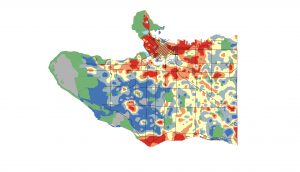
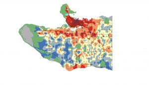 Above: Two examples of the output raster surfaces of the areal interpolation tool in ArcMap. The top map is percentage of renters, where blue tones indicate low percentages and red tones indicate higher. The bottom is the mapped rate of sustainable mode share in commutes for work (walking + biking + transit use) including the location of current and near-future rapid transit stations indicated as blue diamonds. Orange here indicates more than 50% and red indicates more than 69%. Note how areas surrounding transit stations like Marine Drive Station, Broadway-City Hall, Commercial-Broadway, and the entire Downtown Peninsula exhibit very high rates of active/sustainable mode share, as one would expect.
Three additional raster surfaces were created to calculate the distance of spaces in the city to rapid transit stations, schools, and community centres. These were created using a Spatial Analyst tool in ArcMap called Euclidean Distance.
For the multi-criteria evaluation, the values of the raster surfaces had to be converted to a 0-1 scale, with 1 representing ideal targets and 0 representing areas to exclude from the result of the multi-criteria evaluation. To do so, the Raster Calculator tool was used to fit variables such as median commute time to a 0-1 scale, and to invert them when necessary (as in the case of median commute times and distance to nearest transit station) such that lower values (short commutes and short distances that represent the ideal) are represented by values closer to 1.
Using the Weighted Sum Spatial Analyst tool in ArcMap, a raster surface was created to scale space in the city on the basis of these criteria. As a sensitivity analysis, another raster surface was made on the basis on equal weights (0.125 for each criteria). Using the Reclassify tool, the final raster surfaces for the multi-criteria evaluation were created using only the cells whose values superceded 2 standard deviations above the mean value of each surface.
Queries for Target Zones
In preparation for the final stage, I created a polygon layer with the Union tool that included the boundaries of both the dissemination areas and the zoning areas, and their attributes. There are two benefits of having done this. The first is ensuring greater precision in the identification of “zones,” since dissemination areas are in general much smaller in surface area than the largest single-family housing zones. The second is that this makes it possible to verify the final identified zones with the original census data using the dissemination-area ID that would be associated with the final polygons.
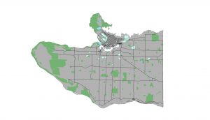
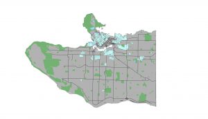
Above: the top image displays the polygon created from the final raster of areas that scored 2 standard deviations and above in the weighted MCE. The bottom image displays the zones-DA union polygons that intersected with the final MCE polygon.
To identify single and two-family zoned areas that overlapped with the final MCE raster, I first converted the raster (of the weighted MCE only) to a polygon using conversion tools. Then, using Select by Location, I queried for the polygons in the unioned zone-DA layer that intersected with the MCE polygon. With these selected, I made a new layer of the selected features, and of those, I selected by attribute using the boolean query CATEGORY = SINGLE-FAMILY OR CATEGORY = TWO-FAMILY and was able to identify the final zones.