472 – Interactive Visualisations – Vancouver Crime Data 2005
For this assignment we were tasked with creating an interactive map that can be posted online to visualise Vancouver Crime data. Cleaning and filtering the raw crime data for the map was conducted using the open source R coding language and RStudio software, and the actual maps were produced using the add-on package ‘leaflet’ (https://rstudio.github.io/leaflet/). To tackle this assignment I followed Ben Fry’s data visualisation pipeline and I will use this framework to explain how my R code converts the original data set into an interactive map. To avoid repeating computer intensive tasks, I separated my code after geocoding the dataset and after offsetting the coordinates. This produced 3 parts that can each be ran separately, as each part first loads the final data output from the previous part.
Section 1: This first section of code installs the packages of functions that are used later in the code. Each time RStudio is reopened, these packages need to be loaded using the function ‘library(package name)’.
##############################################################################
# 472 Assignment 4 - Visualising Vancouver Crime Data
# Date: 20/10/2016
# By: Matthew Wagstaff
# Desc: Take Vancouver Crime Data, clean (subsetting for only 2005 data),
# geocode the addresses and visualise the crime categories
# following the data visualisation pipeline:
# (acquire, parse, filter, mine, represent, refine, interact).
#
# NOTE: Can run each of the three parts of the script separately as long as libraries
# are loaded each time RStudio is restarted.
##############################################################################

#### ---------------------- Install Libraries ------------------------- ####
# run this section once to install the libraries of functions necessary for this code
install.packages("GISTools")
install.packages("RJSONIO")
install.packages("rgdal")
install.packages("RCurl")
install.packages("curl")
install.packages("leaflet")

#### ------------------------ Load Libraries -------------------------- ####
# loads functions from these libraries
library(GISTools)
library(RJSONIO)
library(rgdal)
library(RCurl)
library(curl)
library(leaflet)
Section 2 – ACQUIRE:
The first step is to download the Vancouver crime data and subset for just the 2005 data. The data was downloaded from: https://blogs.ubc.ca/advancedcartography/files/2015/08/crime_csv_all_years_nolatlong.zip
#### ------------------------------------------------------------------------------- ####
#### ---------- **PART 1**: Acquire, clean and geocode data ----------- ####

#### -------------------- ACQUIRE (& Subset Year) --------------------- ####
# load Vancouver Crime data
# (downloaded from https://blogs.ubc.ca/advancedcartography/files/2015/08/crime_csv_all_years_nolatlong.zip)
fname <- 'crime_csv_all_years_nolatlong.csv' # Define filename
data <- read.csv(fname, header=T) # Read the csv and create dataframe
rm(fname) # remove unnecessary variables to keep environment clean

# inspect data
View(data)
# SUBSET DATA FOR JUST MY ASSIGNED YEAR - 2005
data <- data[which(data$YEAR == 2005),]
Section 3 – PARSE (A):
Cleans the 2005 crime data by converting the address data into full addresses in the correct format.
#### --------------------- PARSE: Data Cleaning ----------------------- ####
# Certain crimes do not have associated locations and are listed
# as "OFFSET TO PROTECT PRIVACY" - remove these rows as they can't be mapped
raw_data <- data # create a backup data frame of the original data in the environment
data <- data[which(data$HUNDRED_BLOCK != "OFFSET TO PROTECT PRIVACY"),] # remove rows with code
length(raw_data$TYPE) - length(data$TYPE) # returns number of records removed

# To hide exact address, data is generalised to hundred blocks but is
# formatted with XX for the 00s in the hundred block.
# Change intersection XX's to 00's so can create full address
data$h_block = gsub("X", "0", data$HUNDRED_BLOCK)
print(head(data$h_block)) # check results

# Create column called full_address with hundred block names
# and add "Vancouver, BC" to the addresses.
data$full_address = paste(data$h_block, "Vancouver, BC", sep=", ")

# Changing '/' for 'and' to depict intersections in full_address entries
# (to match formatting from previous geocoding and ensure geocoding function runs)
data$full_address = gsub("/", "and", data$full_address)

#### GEOCODING FUNCTION THAT CALLS THE BC GOVS GEOCODING API ####
Joey Lee’s geocoding function is defined here in the script but I have omitted that text here. The function can be found at https://allthisblog.wordpress.com/2016/10/10/r-with-leaflet-vancouver-311-tutorial/.
Section 4: PARSE (B):
Geocodes the data by sending the addresses to the BC Government’s geocoding API (using the bc_geocode R function written by Joey Lee) and returns coordinates for each crime record. As the geocoding function requires a lot of computing power and time, the data file was written out to a CSV file at the end of this section to prevent having to re-run this section of code when coming back to RStudio.
#### ---------------- PARSE - Geocode the Crime Data ------------------ ####
# Geocode the events using the BC Government's geocoding API

# Create empty vectors for lat and lon coordinates
lat <- c()
lon <- c()

# loop through the addresses
for(i in 1:length(data$full_address)){
# store the address at index "i" as a character
address <- data$full_address[i]
# append the latitude of the geocoded address to the lat vector
lat <- c(lat, bc_geocode(address)$lat)
# append the longitude of the geocoded address to the lon vector
lon <- c(lon, bc_geocode(address)$lon)
# at each iteration through the loop, print the coordinates to update user on progress
print(paste("#", i, ", ", lat[i], lon[i], sep = ","))
}

# add the lat lon coordinates to the dataframe
data$lat <- lat
data$lon <- lon

# save the data as .csv
write.csv(data, "Crime_Data_Geocoded.csv")
Section 5 – FILTER:
Filters the data for only the points within the bounds of the City of Vancouver that were geocoded with valid coordinates. After visualising the data to check the distribution using the plot function, it was clear for viewers with knowledge of Vancouver that a few data points were plotted in North Vancouver. It appears this was a mistake by the geocoding function and these points were plotted on the wrong Main Street, so these records were also removed from the data and a new data frame saved as CSV.
#### ------------------------------------------------------------------------------- ####
#### -------------- **PART 2** - Load Data from Part 1 ---------------- ####
file_loc <- "Crime_Data_Geocoded.csv"
data <- read.csv(file_loc, header = TRUE)
rm(file_loc)

#### ------------ FILTER: Locations only within City of Vancouver ------------- ####

# Subset to only keep data with coordinates within Vancouver and not NAs
data_filter = subset(data, (lat <= 49.313162) & (lat >= 49.199554) &
(lon <= -123.019028) & (lon >= -123.271371) & is.na(lon) == FALSE)

# plot the data to check distribution
plot(data_filter$lon, data_filter$lat)

### Some points have been geocoded in North Vancouver - remove them
# subset a list of these points
North_Van = subset(data_filter, (lat >= 49.3) & (lon >= -123.06))
# remove points from data_filter that are in the north van subset
North_Van_Removed <- data_filter[-which(data_filter$lat %in% North_Van$lat),]
# plot again to re-check the distribution
plot(North_Van_Removed$lon, North_Van_Removed$lat)

# If everthing looks good, write out the file and overwrite data:
data <- North_Van_Removed
rm(data_filter, North_Van_Removed, North_Van)
write.csv(data, "Crime_Data_2005_Geocoded_Filtered.csv")
Section 6 – MINE:
In this section I examined the categories that the crime data was classified as, and as there are only six categories, decided to include all six categories on the interactive map. Because the locations of the crime records were generalised to hundred block, many of the points have the same exact location, and so a for loop was included in the code to take each crime record, and if it has the same location as another record, offset it’s location by a small amount. This ensures that points will not be mapped on top of one another and all points will be visible. Again to avoid having to repeat this section, the file is then written out as a CSV. The last code chunk of this section outputs a list of the frequency of each crime type in descending order.
#### ----- MINE: Classify data and add jitter to avoid overlapping ---- ####

# Examine unique crime types
unique(data$TYPE)

### Only 6 Crime types so will leave ungrouped and create check layers so you can
### select multiple layers together, such as both the residential and commercial
### break & enter categories

### Calls are generalised to hundred block so need to handle overlapping points
# Create columns to offset coordinates of points in same location:
data$lat_offset = data$lat
data$lon_offset = data$lon

# Loop to offset any overlapping values by a random number between 0.0001 and 0.0005
for(i in 1:length(data$lat)){
if ( (data$lat_offset[i] %in% data$lat_offset) && (data$lon_offset[i] %in% data$lon_offset)){
data$lat_offset[i] = data$lat_offset[i] + runif(1, 0.0001, 0.0008)
data$lon_offset[i] = data$lon_offset[i] + runif(1, 0.0001, 0.0008)
}
}
rm(i)

# plot the data to check results
plot(data$lon_offset, data$lat_offset)

# if results look good, write out the file:
write.csv(data, "Crime_Data_2005_Geocoded_Filtered_Offset.csv")

# Explore the crime type - frequency distribution of the calls:
top_crimes = data.frame(table(data$TYPE))
top_crimes = top_crimes[order(-top_crimes$Freq), ]
print(top_crimes)
Section 6B:
The next section of code takes the geocoded dataframe and converts and saves the data as shapefiles and GeoJSON for use with other software and GIS programs outside of R.
#### --------- Convert and Save Data to Shapefile & GeoJSON ----------- ####
# store just the coordinates in dataframe
Crime_Coords = data.frame(data$lon_offset, data$lat_offset)

# create spatialPointsDataFrame
data_shp = SpatialPointsDataFrame(coords = Crime_Coords, data = data)

# set the projection to wgs84
projection_wgs84 = CRS("+proj=longlat +datum=WGS84")
proj4string(data_shp) = projection_wgs84

# set an output folder for geojson files and join to each file name::
geofolder = "R/GEOB472/"
opoints_shp = paste(geofolder, "VanCrime2005", ".shp", sep = "")
opoints_geojson = paste(geofolder, "VanCrime2005", ".geojson", sep = "")

# Write data out as shape file
writeOGR(data_shp, opoints_shp, layer = "data_shp", driver = "ESRI Shapefile",
check_exists = FALSE)
# write data out as geojson
writeOGR(data_shp, opoints_geojson, layer = "data_shp", driver = "GeoJSON",
check_exists = FALSE)
ASIDE: Process Notes
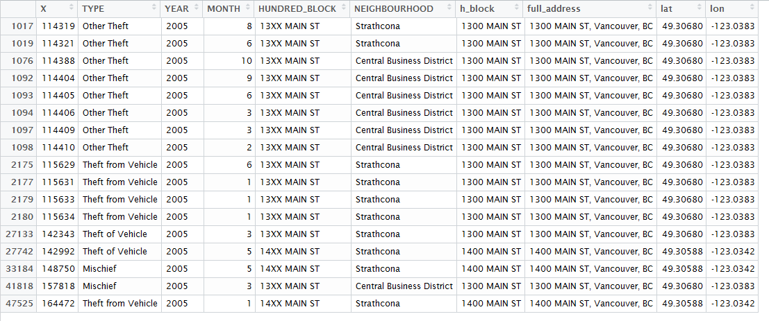
Throughout the process of cleaning the data, some records are lost at each step. The raw crime data file contained 576,876 records, with 51,397 occurring in 2005. 3,791 had had their locations hidden for privacy reasons and removing these reduced the total to 47,606 records. A further 55 records were removed by the filtering function which removed any records with NA coordinates or coordinates which were not within a defined rectangle that represented the coordinates of the City of Vancouver. At this stage when the data was plotted to check the distribution, I noticed a number of records that didn’t match the expected geographic pattern and appeared to be located across Burrard inlet in North Vancouver. After filtering for these records, 17 observations were found to have been geocoded as in North Vancouver. It appears this may have been a result of an error within the geocoding function as the records accompanying data showed they should have been placed on Main Street in East Vancouver or Strathcona, but had instead been placed on the wrong “Main Street” – across the inlet. See the records in the top right corner of the preliminary plot below (this step is before the points were offset from one another so appear as just 2 points) and the screenshot of the data frame. After removing these records, a final total of 47,534 records remained. 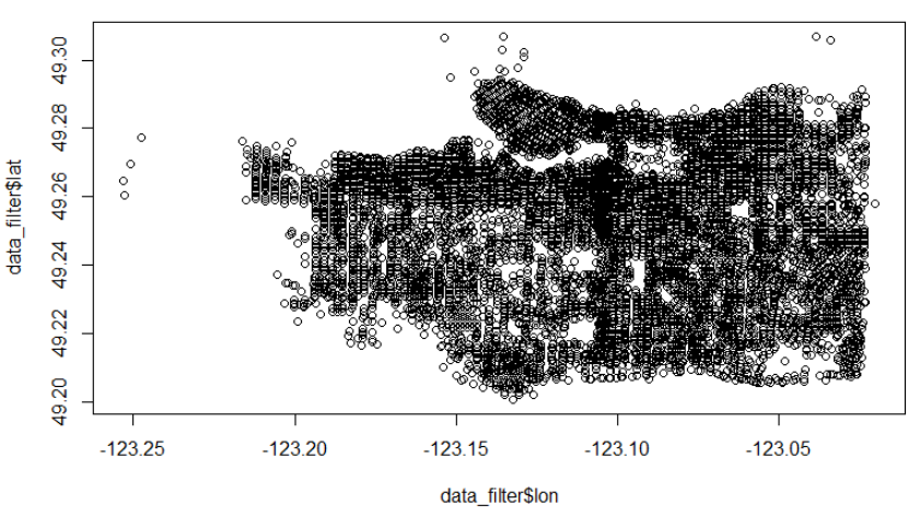
While the 3,791 records with their records removed constitute a fair amount of error (7% of the total 2005 data), the process itself found little further error in the data, with only 72 records having to be removed (0.15% of the remaining records). While a number of these removals (the North Vancouver records and potentially some of the other 55 removed for being outside of Vancouver or NA locations) may have been caused by mistakes in the geocoding process, this is a very small fraction of the data set. Overall I conclude that the data set appears to be reliable but the 7% of records that are hidden could potentially bias the results of any analysis conducted on this data.
The frequency of the six crime types in this final data set was as follows (descending order):
- Theft from Vehicle: 16,529
- Other Theft: 12,764
- Break and Enter Residential/Other: 5,527
- Mischief: 5,052
- Theft of Vehicle: 5,024
- Break and Enter Commercial: 2,638
File Formats
At the end of this data cleaning and preparation process I saved the shape data in two different formats: ESRI’s shapefile format, and GeoJSON. While the two formats contain the same data in this case, they store that data in different ways. The ESRI ARC Shapefile format is the standard for the popular ArcGIS software suite and stores different information about the shape in multiple files with formats including: .shp, .shx, and .dbf. In contrast, GeoJSON files are an open standard where all the information about the shape is stored in one .geojson file; this makes the shapefile easier to edit and use online, but with the drawback that the one file cannot contain all the information that can be stored in an ARC Shapefile such as any styling information as to how to portray the shape. I chose to output both formats as they are two of the most commonly used formats in the industry and allow for further work with this dataset in other software. If I was planning to conduct further geographical analysis and had access to ArcGIS software, I would use the ARC shapefile, whereas for this project I use the GeoJSON files later in the script as they are easier to work with and easier to portray online.
Now back to the code….
Section 7 – REPRESENT (Preparation):
In this, the final step before mapping using the leaflet package, I import a hex grid polygon layer that was created by Joey Lee, and use the poly.counts function to count the number of crimes per hexagon shell in order to be able to visualise crime density on our maps. This hexagon density layer is then also saved as a shapefile and GeoJSON.
#### -------- REPRESENT: Aggregate to Grid & Save Shape Files --------- ####
# ref: http://www.inside-r.org/packages/cran/GISTools/docs/poly.counts
# set file name & read in hex grid
grid_fn = 'hgrid_250m.txt'
hexgrid = readOGR(grid_fn, 'OGRGeoJSON')
rm(grid_fn)

# transform the projection to wgs84 to match the crimes file and store
# as new variable (see variable: projection_wgs84)
hexgrid_wgs84 = spTransform(hexgrid, projection_wgs84)
# Use the poly.counts() function to count the number of crimes per grid cell
grid_count = poly.counts(data_shp, hexgrid_wgs84)
# create a data frame of the counts
grid_total_counts = data.frame(grid_count)
# set grid_total_counts dataframe to the hexgrid data
hexgrid_wgs84$data = grid_total_counts$grid_count
# remove all the grids without any calls
hexgrid_wgs84 = subset(hexgrid_wgs84, grid_count > 0)
# define the output names:
ohex_shp = paste(geofolder, "VanCrime2005_250mHexgrid_Counts", ".shp", sep = "")
ohex_geojson = paste(geofolder, "VanCrime2005_250mHexgrid_Counts", ".geojson", sep = "")
# write the file to a shp
writeOGR(check_exists = FALSE, hexgrid_wgs84, ohex_shp,
layer = "hexgrid_wgs84", driver = "ESRI Shapefile")
# write file to geojson
writeOGR(check_exists = FALSE, hexgrid_wgs84, ohex_geojson,
layer = "hexgrid_wgs84", driver = "GeoJSON")
Section 7B:
In addition to this hexagon layer that has been created to visualise crime density across the city, I also wanted to visualise the crime density relative to more recognisable areas. To do this I downloaded shapefiles from the City of Vancouver website (http://data.vancouver.ca/datacatalogue/localAreaBoundary.htm) of the local area boundaries within the city, imported them into R and performed the same process as with the hex layer to create a second crime density layer.
#### --- REPRESENT 2: Aggregate to LOCAL AREAS & Save Shape Files ----- ####
# shapefiles source: http://data.vancouver.ca/datacatalogue/localAreaBoundary.htm
# set file name & read in Local Area Boundaries
LA_folder = 'local_area_boundary_shp'
LAs = readOGR(LA_folder, 'local_area_boundary')
rm(LA_folder)

# transform the projection to wgs84 to match the crimes file and store
#  as new variable (see variable: projection_wgs84)
LAs_wgs84 = spTransform(LAs, projection_wgs84)
# Use the poly.counts() function to count the number of crimes per Local Area
LAs_count = poly.counts(data_shp, LAs_wgs84)
# create a data frame of the counts
LAs_total_counts = data.frame(LAs_count)
# set LA_total_counts dataframe to the LA data
LAs_wgs84$data = LAs_total_counts$LAs_count
# remove all the grids without any calls
LAs_wgs84 = subset(LAs_wgs84, LAs_count > 0)
# define the output names:
LAs_shp = paste(geofolder, "VanCrime2005_LocalAreas_Counts", ".shp", sep = "")
LAs_geojson = paste(geofolder, "VanCrime2005_LocalAreas_Counts", ".geojson", sep = "")
# write the file to a shp
writeOGR(check_exists = FALSE, LAs_wgs84, LAs_shp,
         layer = "LAs_wgs84", driver = "ESRI Shapefile")
# write file to geojson
writeOGR(check_exists = FALSE, LAs_wgs84, LAs_geojson,
         layer = "LAs_wgs84", driver = "GeoJSON")
Section 8 – REPRESENT – Web Mapping:
Finally, time to make maps! As you can see preparing the data ready for creating maps and visualisations can often take significantly more time than creating the visuals themselves. In this final part I read in the prepared data and create maps using the leaflet package. The first section of code creates a simple map with point layers for each crime type. The first step to do this is to categorise the crime records based on the crime type by subsetting the data, and then adding a colour function from which to add colours to each crime type layer. Then the next steps are to initiate a leaflet map and add map layers and point layers for each of the crime types.
#### ------------------------------------------------------------------------------- ####
#### -------------- **PART 3** - Load Data from Part 2 ---------------- ####
# read in our final data file from Part 2
filename = "Crime_Data_2005_Geocoded_Filtered_Offset.csv"
data = read.csv(filename, header = TRUE)
rm(filename)

#### -------- REPRESENT: Subset and map just crime point layers ------- ####
# Create list with subsets of each crime category to loop through
data_subset_list = list(df_BE_C = subset(data, TYPE == "Break and Enter Commercial"),
                       df_BE_RO = subset(data, TYPE == "Break and Enter Residential/Other"),
                       df_TOV = subset(data, TYPE == "Theft of Vehicle"),
                       df_TFV = subset(data, TYPE == "Theft from Vehicle"),
                       df_OT = subset(data, TYPE == "Other Theft"),
                       df_M = subset(data, TYPE == "Mischief"))

# Create list of layers:
layerlist = c("1 - Break & Enter - Commercial", "2 - Break & Enter - Residential/Other",
              "3 - Theft of Vehicle","4 - Theft from Vehicle", "5 - Other Theft",
              "6 - Mischief")

# create colour palette based on crime type
colorFactors = colorFactor(c('brown', 'red', 'orange', 'purple', 'blue', 'pink'),
                           domain = data$TYPE)

# initiate leaflet
m = leaflet()

# add open street map and toner lite background map tiles
m = addTiles(m, group = "OSM (default)")
m = addProviderTiles(m, "Stamen.TonerLite", group = "Toner Lite")

# Loop through crime types and add markers to map for each
for (i in 1:length(data_subset_list)){
  m = addCircleMarkers(m,
                       lng=data_subset_list[[i]]$lon_offset, # feed the longitude coordinates
                       lat=data_subset_list[[i]]$lat_offset, # lat coords
                       popup=data_subset_list[[i]]$TYPE,     # what to popup
                       radius=2,                             # radius of circle
                       stroke = FALSE,                       # no outline
                       fillOpacity = 0.75,                   # opacity of circle
                       color = colorFactors(data_subset_list[[i]]$TYPE), # fill colour of circle based on type
                       group = layerlist[i]                  # name the group
  )
}

# add layer control function to map - base maps are toner lite and open street map,
#   and function as radio buttons, while crime layers are overlay groups with check boxes to map them
m = addLayersControl(m,
                     baseGroups = c("Toner Lite","Open Street Map"),
                     overlayGroups = layerlist)

# make the map
m
Section 9 – REFINE & INTERACT – Interactive Web Mapping
After this first simple map, I refined the code to produce a final interactive map. After initiating a new leaflet map, I added two background map options, Open Street Map and a simple grey and white theme, then added the crime density hexagon layer, the local area crime density layer and the point layers for each crime type. A red colour palette with continuous values is created along with a legend to allow for the visualisation and interpretation of the hex crime density layer (red was chosen as crime is a negative factor) and a blue colour palette is created for the local area crime density layer along with an accompanying legend. The colours for each of the crime type layers are also individually set using hex codes obtained from a chosen colour scheme on http://colorbrewer2.org. To improve on the previous colour scheme, I grouped the similar categories into similar colours, with both Break & Enter categories a shade of purple, Thefts a shade of green, and more serious vehicle thefts and lower severity mischief orange and blue respectively. To make the map interactive, the function addLayersControl() is used to allow the user to choose which layers are shown on the map. For this map, the two background map options were added as base layers which are selected using radio buttons, and then the crime density hexagon layer and the crime type points were added as overlay groups which can be added as check layers (allowing the user to choose which layers to overlay on the chosen base map). Each of these layers also had popup features so when a hexagon or a point is clicked on, the number of crimes in that hexagon or the crime type of the point pop up over the map. Finally, to save the map for online use, the user can click on the export option within the map viewer and choose to export the map as a .html file, which can then be opened in any web browser or hosted online.
#### --------------- REFINE: Create New Map with Layers --------------- ####
# initiate leaflet map and add open street map and simple toner map tiles
m = leaflet()
m = addTiles(m, group = "OSM (default)")
m = addProviderTiles(m, "Stamen.TonerLite", group = "Toner Lite")

# load the geojson hex and Local Areas grids
hex_crime_fn = 'VanCrime2005_250mHexgrid_Counts.geojson'
hex_crime = readOGR(hex_crime_fn, "OGRGeoJSON")
LAs_crime_fn = 'VanCrime2005_LocalAreas_Counts.geojson'
LAs_crime = readOGR(LAs_crime_fn, "OGRGeoJSON")

# Create a continuous colour palette of reds for the hex grid and blues for
# the Local Areas based on the crime density
HEXpal = colorNumeric(palette = "Reds", domain = hex_crime$data)
LApal = colorNumeric(palette = "Blues", domain = LAs_crime$data)

# add hex grid to m coloured by the crime density using the HEX palette
m = addPolygons(m,
                data = hex_crime, # data
                stroke = FALSE,   # no outline
                smoothFactor = 0.2, # smoothing of shapes
                fillOpacity = 1,    # opacity
                color = ~HEXpal(hex_crime$data), # colour function to assign shade of red based on crime count
                popup= paste("Number of Crimes: ",hex_crime$data, sep=""), # text to pop up when clicked on
                group = "City Crime Density"  # give group name to this layer
)

# add Local Areas grid to m coloured by the crime density using the LA palette
m = addPolygons(m,
                data = LAs_crime, # data
                stroke = FALSE,   # no outline
                smoothFactor = 0.2, # smoothing of shapes
                fillOpacity = 1,    # opacity
                color = ~LApal(LAs_crime$data), # colour function to assign shade of red based on crime count
                popup= paste(LAs_crime$NAME, " - Number of Crimes: ",LAs_crime$data, sep=""), # text to pop up when clicked on
                group = "Local Area Crime Density"  # give group name to this layer
)

# add legends for the crime density colours
m = addLegend(m, "bottomright", pal = HEXpal, values = hex_crime$data,
              title = "Annual Crime Density",
              labFormat = labelFormat(prefix = " "),
              opacity = 0.75
)
m = addLegend(m, "bottomleft", pal = LApal, values = LAs_crime$data,
              title = "Local Area Crime Density",
              labFormat = labelFormat(prefix = " "),
              opacity = 0.75
)


### Add Crime Type Layers ###
# IMPROVED COLOUR PALETTE from last map - hex codes selected from colorbrewer2.org
colorFactors = colorFactor(c('#7b3294', '#c2a5cf', '#0571b0',
                             '#008837', '#a6dba0', '#fdb863'),
                           domain = data$TYPE)
# Break and Enter categories are 2 different shades of purple
# Theft from Vehicle and Other theft are 2 shades of green
# Theft of Vehicle - orange
# Mischief - blue

for (i in 1:length(data_subset_list)){
  m = addCircleMarkers(m,
                       lng=data_subset_list[[i]]$lon_offset, # feed the longitude coordinates
                       lat=data_subset_list[[i]]$lat_offset, # lat coords
                       popup=data_subset_list[[i]]$TYPE,     # what to popup
                       radius=2,                             # radius of circle
                       stroke = FALSE,                       # no outline
                       fillOpacity = 0.75,                   # opacity of circle
                       color = colorFactors(data_subset_list[[i]]$TYPE), # fill colour of circle based on type
                       group = layerlist[i]                  # name the group
  )
}

#### -------------- INTERACT: add layer control features -------------- ####
m = addLayersControl(m, baseGroups = c("Toner Lite", "Open Street Map"),
                     overlayGroups = c("City Crime Density", "Local Area Crime Density", layerlist))
# base groups are radio buttons - set based maps
# overlay groups are selectable layers - set crime density hex's and markers

# show map
m

# To output this map as a .html file that can be viewed online, choose the export option
#  in the viewer window.
Unfortunately WordPress does not support embedding .html files such as the final interactive map so here is a link to the file (requires download of the file to open):
https://dl.dropboxusercontent.com/u/43982661/VanCrime2005_Matt_Wagstaff.html
In addition, here are some screenshots of the final product:
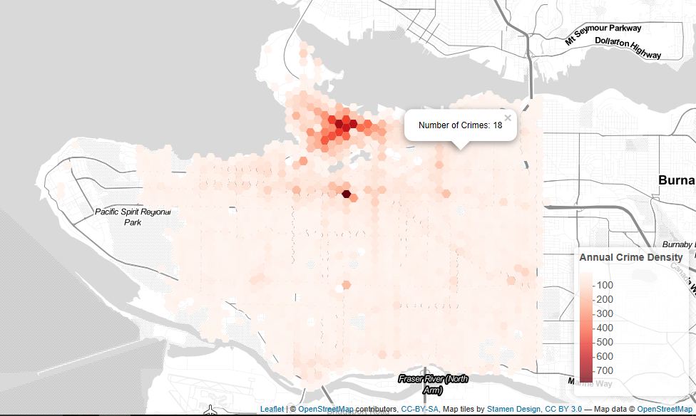
Crime Density Hexagon Layer – with legend and pop up example
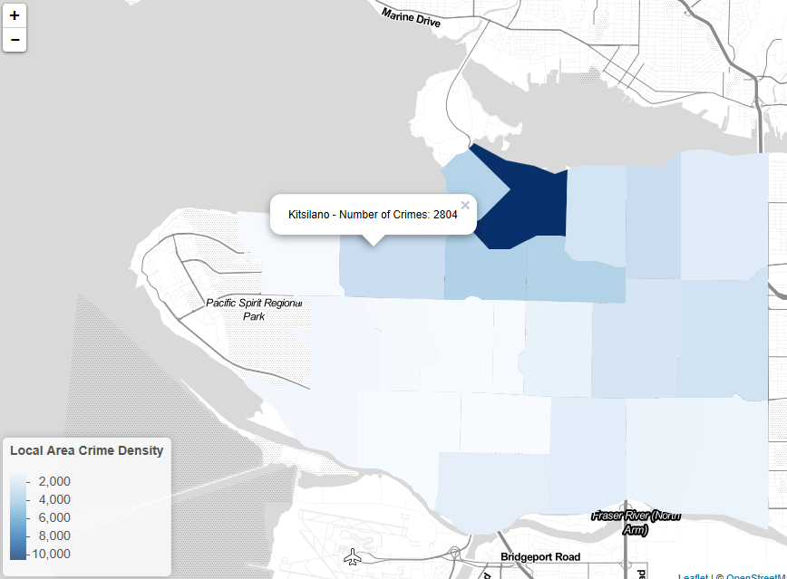
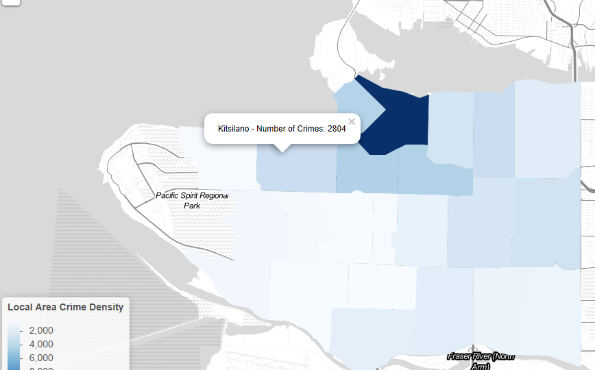
Local Area crime density layer with legend and pop-ups on click to identify local area and number of crimes that occurred in 2005.
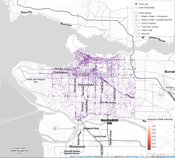
Both Break & Enter Categories Selected
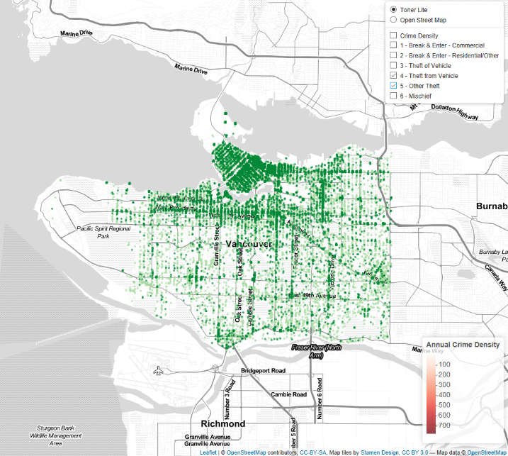
Both Normal Theft Categories Selected
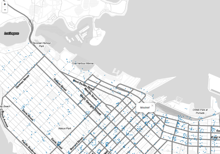
Zoomed in section with Mischief category selected, pop up functionality of each point demonstrated.
Visualization Notes:
Cartographic Constraints:
As a relative newcomer to using R, and a complete beginner in terms of using R to interpret and visualise spatial information, there is a steep learning curve to working with this software. Learning to utilise a coding language effectively is no different than having to learn how to speak a completely new language. Therefore it was difficult to write the code to produce the exact cartographic elements I wanted. While I was able to produce the map elements that I wanted, there was certain details of different map layers that I was unable to set as I wanted. Specific examples would be the colour palettes used for the two crime density layers, and the outline of the local area boundaries. While the final colour palettes are successful in visualising crime density, I would have chosen to start them at a light shade of the colour, rather than at white, so the lowest density polygons are more visible on the white base layer of the map. For the outlines of the polygons, I was able to add them to the local area polygons, but was unable to figure out how to edit them to a format I liked and so ended up removing them to keep the map’s clean appearance. With further understanding of the leaflet package, I would also add a title, scale (that adjusts with zoom) and information about my data sources etc so the user can see where my data is from – as well as including a link to my code that I used to create the map so a user can see how the map was produced if they are interested and understand what assumptions and decisions I made when presenting the data.
Visualisation Insights
I believe the interactivity of this visualisation is very useful in enabling the user to be able to look at the specific crime types that they are interested and explore the associated spatial patterns. In an ideal world where I am a more accomplished programmer, I would like to add the functionality where you can choose the data you want to visualise such as the year of data (or total over the length of the data set), the crime types (ie. total crimes or just break and enter), and then choose the format you want this data to be visualised in, for example, point layer of each record, density layer by local areas, or a density layer across the whole city such as Joey Lee’s hex layer.
The local areas density layer was successful in giving an initial overview of the data and values to compare each area. This layer clearly shows the increase in crime density in areas closer to the downtown core. This makes logical sense as these are the areas with higher population density but you would also expect them to have higher rates of policing. The hex layer is then more specific with greater resolution and shows you interesting trends such as the hotspot around City Hall (Broadway and Cambie Street), and the high crime density along Granville and Georgia streets downtown. Finally the point layers of each crime type showing all records allows you to directly visualise the data and where crimes occur. When exploring patterns in these point layers it is possible to draw conclusions about their distribution, such as how break and enters of commercial properties are only located on main through roads because that is where commercial properties are concentrated. However, the sheer volume of points in these point layers can be overwhelming and difficult to draw out patterns, so creating layers such as the density layers included on the map allows the user to visualise this data more simply. If you were to create a visualisation of a data set with more records, for example crime over the decade rather than just 2005, I don’t think these point layers would be useful (and would significantly slow most computers due to the volume of points) and instead I would plot density layers for each crime type.
Reflection – Proprietary Software vs Free Open Source Software (FOSS):
Most university programs teach the technical aspects of geospatial analysis and cartography using proprietary software packages that have become the industry standards such as ESRI’s ArcGIS and Adobe Illustrator. These programs are very powerful and have been developed and refined over many years to be efficient tools. However due to their nature, this software is very expensive for an individual or infrequent user to access, and so when students lose access to these programs through their university, they often are unable to utilise their skills unless they are employed by a company that can afford these software programs. FOSS is different in that by definition it is open and free to use for anyone. As well as giving anyone access to use these powerful software tools – which clearly has many benefits, the open source nature of these software tools allows for fast development and improvement of these tools. Experienced software developers can write complimentary programs and packages for these FOSS and help users to accomplish tasks that weren’t possible before or at least simplify them and speed up workflows. For this same reason, there is also a lot of information and resources online to help new users learn to use and troubleshoot problems with these software programs. The fact that anyone has access to these programs allows users to share for example their R code or the methods they used in QGIS to conduct a project, so that others can understand how the final project was produced, what data was used, what assumptions had to be made and whether any errors may have been made along the way. It also allows for collaboration and lets other people expand and improve projects if you choose to make them public (for example feel free to improve on my Vancouver Crime map!). As long as these FOSS programs are well maintained, I do not see any cons to their increased use.