RCP 8.5 vs. RCP 2.6

This analysis shows just how huge of a difference strong mitigation or business as usual measures can have on the wellbeing of coastal communities. The likelihood of flooding maps show that a business as usual scenario would lead to far more flooding along the coast than the strong mitigation scenario, and would essentially erase Miami Beach’s footprint. Furthermore, flooding from coastal inlets impacts much more of the city center of Miami, as well as urban areas near the Miami-Dade coast.

The suitability models for sea level vulnerability show a similar pattern; in an RCP 8.5 scenario, vulnerable areas appear to be more than doubly frequent than an RCP 2.6 scenario, regardless of whether the weight is on physiographic or socioeconomic factors. The visual sensitivity analysis shows that the RCP 2.6 scenario would largely keep vulnerable areas to the immediate coastline, while the RCP 8.5 scenario has the effect of rendering almost the entirety of the cities of Miami and Miami Beach highly vulnerable, and vulnerability extends far into the coastline of much of Miami-Dade County.

Areas of Vulnerability

The results of the analysis can be “ground-truthed,” to a certain extent, with some research into the communities that the analysis deems vulnerable. Little Haiti, a historically black and very condensed community, is shown as highly vulnerable on the maps, validating the methodology used. However, it is crucial to note that perceived vulnerability can often be far from actual vulnerability; that is to say, the adaptive capacity of a community is not only reliant on the social factors discussed, but also on the social behaviours of a community itself. For example, Little Haiti is highly condensed and may therefore be seen as difficult to escape in flooding events; however, there could be cultural practices that are unknown outside the community that mitigate this.

 

Figure 14. Little Haiti neighbourhood in Miami

Irregularity in Suitability Next To Coastlines

One area of interest is the irregularity in some coastal raster cells in the suitability model. As can be seen in figure 15, some pixels right on the coastline are seen as being ‘not suitable’ for vulnerability of sea level rise (greener shades). When considering this dilemma (after all, distance from coastline was a defining factor of suitability), the architectural structures of Miami-Dade coastlines are important. Miami-Dade is famous for sandy beaches and blue waters that have made it an appealing place for high-rise apartment buildings to be built, allowing as many people to live next to the water as possible. As a result, despite the smoothing processes performed on the DEM, these areas retain a ‘high’ elevation, even though the bases of the buildings are at sea level.

Seen below is a section of the Suitability Model of RCP 2.6 with a focus on the physiographic variables. Paired with it are two screenshots taken from GoogleEarth; one in 2D and one in 3D.

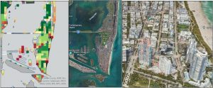
Figure 15. Miami Beach represented in the formats of a suitability model output, and a GoogleEarth 2D image, and the Southern tip of Miami Beach represented in the format of a GoogleEarth 3D image

There is irregularity in the vulnerability of Miami Beach, despite it having low elevation and being surrounded by water, as can be seen in the 2D image from GoogleEarth. One explanation for the model’s decision can be seen in the 3D image from GoogleEarth, displaying the Southern tip of Miami Beach. What can be noticed is that the buildings in this location are multi-story, high-rise apartment buildings. These buildings are also large, some of them the same size as an individual raster cell, explaining how there can be such variability between neighbouring raster cells in locations of presumed high-vulnerability.

Subsequently, given the high weight placed on elevation throughout the modelling process, the raster cells containing these buildings of high total elevation are seen to be ‘not suitable’ for sea level rise vulnerability, despite the reality being that the lower levels of these buildings are as susceptible to sea level rise as their lower total elevation neighbours. Furthermore, the likelihood map shows with 100% confidence that this area will not be flooded, but the actual ground level elevation is the same as the south-west coast, which is shown as 100% likely to be completely submerged.

Uncertainty

There are many sources of uncertainty in this analysis to consider. One overarching source of uncertainty is the resolution of the created raster surfaces, which all had to be different owing to technological constraints (such as the time to perform processes, the resolution that tools could handle, and the resampling process for the generated DEM). Additionally, every time surfaces are resampled or other processes are performed to make them suitable for the purposes of a project, even more uncertainty is inherently introduced in the computation. The likelihood of flooding maps are only suitable for visual reference along the coast-line, and area-based calculations were not used in this process for the following reasons: a) the likelihood maps do not consider the distance from coastline, so water reservoirs and other low-lying inland areas appear as though they will be flooded; b) the raster cells extend beyond the natural coastline, so any calculation regarding areas would include raster cells that fall within the ocean; and c), the likelihood surface for the RCP 8.5 (0.95 meters of sea level rise) does not show likelihood values between -1 and 1, likely due to the elevation profile of the study area.

Another source of uncertainty in the analysis is the initial DEM. Because no bare-earth DEM was available and the processes performed did not completely eliminate the elevation effects of buildings, it is likely that the analysis underestimated the total coverage of flooding in both scenarios. Furthermore, specification error– or the omission of important variables- is unavoidable in this analysis. The census tract variable proxies for socio-economic vulnerability are only a few of the many dynamic factors that lead to vulnerability, and race, residential density (housing units), and wealth (median household income) are in no way fully representative of people’s adaptive capacities.

There is uncertainty in the spread of raster cells located within the census tract boundaries. When creating the suitability models, multiple layer formats were needed. The socio-economic layers were raster layers that generalised raster cells across the census tract boundaries since the data was per census tract (as downloaded). On the other hand, the DEM and distance from coastline layers were also rasters, but were not limited by census tract boundaries, and were not generalised as the socio-economic layers were; each individual cell has its own unique value. When combining these different layers in the suitability models, the result was that the suitability raster cells took on the characteristics of the physiographic layers, and each raster cell was given its own level of suitability. This meant that census tracts were divided by raster cell size, and there is variability within them.

Interestingly, despite the aforementioned uncertainty, some census tracts retained block characteristics, showing that the physiographic variability within them was uniform. Overall, this creates an interesting visual effect where some areas- the coastlines in particular- have many pixels that are suitable to sea level rise as neighbours, and other areas- mainly inland- retain the census tract block visuals.