- Preliminary research
The first stage of research for this project involved determining the potential sea-level rise scenarios faced by the study area. After reviewing the literature, it was determined that using the year 2100 as a setting for the analysis was appropriate, and building upon established scientific knowledge, two scenarios were chosen for exploration. A strong mitigation scenario, with an RCP (representative concentration pathway) of 2.6, predicts that the likely range of sea-level rise by 2100 is 0.4-0.6m. An unmitigated warming scenario with an RCP of 8.5 predicts a likely range of sea-level rise of 0.7-1.2m by 2100.
Another aspect of the preliminary research involved determining the physiographic determinants of risk, and the socio-economic determinants of vulnerability. With regards to risk factors, having reviewed existing literature specific to the geographic region in question, it was decided that in Miami-Dade county the two most determinative factors of risk are elevation and distance from coastline and water bodies. As such, a DEM (Digital Elevation Model) and a high-resolution coastal polyline were required for the next steps in the analysis.
When determining the social factors that contribute to vulnerability, there was a wealth of existing literature; however, none was specific to Miami-Dade county. Four papers were chosen that explored social factors that determine vulnerability. The results were collated in the table below:
| Factor | Wu et al. | Felsenstein & LIchter | Sales Jr. | Martinich et al. |
| Water Supply | Y | N | N | N |
| Transportation (mobility) | Y | N | N | N |
| Electricity | Y | N | N | N |
| Water Treatment and Sewage | Y | N | N | N |
| Telecommunication | Y | N | N | N |
| Gender | Y | N | N | N |
| Age | Y | Y | N | N |
| Disability | Y | N | N | N |
| Family Structure | Y | N | N | N |
| Housing Units | Y | N | Y | Y |
| Income | Y | Y | Y | N |
| Material Resources (wealth) | Y | Y | Y | Y |
| Race | Y | N | N | Y |
| Ethnicity | Y | N | N | Y |
| Education | N | Y | N | N |
| Insurance | N | Y | N | N |
| Health | N | Y | N | Y |
| Employment | N | N | Y | N |
| Poverty | N | N | N | Y |
This table recorded all the variables discussed in the respective papers, and then noted if they appeared in other papers (Y), or not (N). Basing the choices on the results of the literature, the following three determinants of social vulnerability were chosen to include in the analysis:
- Race
- Median Household Income
- Number of Housing Units
Bearing in mind that this project focuses on Miami-Dade Census Tracts, the data for these variables was US census data. Access to the website ‘Social Explorer’ allowed the downloading of the data in .xlsx format, which could then be easily modified and uploaded to ArcGIS Pro.
2. Creating Usable Surfaces for the Suitability Modeller:
In order to perform the MCE analysis, all of the required data needed to be obtained or created, rasterized, and modified. The steps required for each dataset will be detailed below. All tools and processes used and documented were in ArcGIS Pro.
2.1 Digital Elevation Model
A digital elevation model (DEM) was the most obvious required factor in the MCE analysis; in order to determine whether a location will be at greater risk for flooding as eustatic sea levels rise, one must have a method for comparing the predicted sea levels with the elevation of the land itself. Raw LiDAR imagery was the only available data for the study area, which presented several immediate problems. First and foremost, the LiDAR data presented the elevations in feet, and the rest of the data used had meters as its units. To deal with this, the “raster calculator” tool was used to convert the data by multiplying by 0.3048.
The next complication was that the LiDAR DEM was not a “bare earth” model, so building elevations were more prevalent in the raster than the ground beneath them (which is the factor of interest for sea level rise). In order to reduce the impact that these structures would have on the analysis, the “block statistics” tool with the “minimum” statistics function was used to create a new raster with a coarser resolution (18 meters squared was chosen, because finer pixel sizes did not do enough to reduce the impact of buildings), which displayed the lowest elevation value in the new raster cell. However, before using “block statistics,” the elevation data was multiplied by 10 in order to not lose significant digits in later processes; this was done with the “raster calculator.” Additionally, the “block statistics” tool cannot be used on rasters with “float” data, so the newly multiplied raster was converted to integer data using the “int” tool. After these steps, the multiplied integer raster was put into “block statistics” as described.
To complete the process of creating a usable DEM, the new raster was resampled to 18 meter squared resolution using the “resample” function with the “majority” rule. This ensured that the resulting cells contained only the lowest elevation pixels.
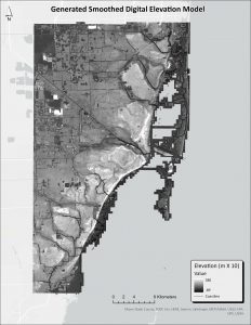
Figure 1. The end result of the DEM smoothing process, shown in 10s of meters. The pixel size of the new DEM is 18 meters.
2.2 Likelihood Surface
With the smoothed DEM, two probability surfaces were generated to reflect the differing probabilities of areas being flooded with different scenarios of sea level rise. To begin, the “fuzzy membership” tool was run with the “gaussian” rule, using the predicted sea level rise as a midpoint (0.5 and 0.95 meters for each RCP scenario respectively). Next, a constant surface raster with values of 1 was generated with the “create constant raster” tool. By subtracting the fuzzy membership raster from the constant raster, the fuzzy membership raster was inverted. Then, the initial unaltered DEM was reclassified so that values scenarios were -1, 0, and 1 were below, at, or above the respective sea level rise of the two RCP scenarios. Finally, the inverted DEM was multiplied by the reclassed DEM raster, producing a usable probability surface.
2.3 Distance to Coastline Raster
To take the distance from the coastline into consideration- because areas further from the coast are at lower risk, regardless of their elevation- a “distance from coastline” raster was created. This required the use of a high resolution polyline shapefile of the coastline of Miami-Dade County. Firstly, a fishnet of the entire study area with 90 meter squared cell size was created using the “fishnet” tool. The centerpoints of every cell were then input into the “euclidean distance” tool to determine how many meters they were from the coast polyline. Then, using the “point to raster” tool, the centerpoints were converted to a 90 meter squared resolution final raster. Note that such a coarse resolution was only selected because the tools were not functioning at a finer resolution.
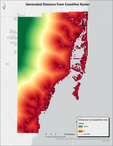
Figure 2. The generated distance from coastline raster (measured in meters), displaying how far pixels are from water boundaries. The pixel size of the raster is 90 meters.
2.4 Rasterizing the Social Variables
The census tract variables of median household income, race, and housing units were rasterized by simply using the “vector to raster” tool three times, with the desired variable as the input values. Note that the race factor was converted to “percent non-white” (using excel) so that only one raster surface was required – the decision to choose this proportion was made in line with the literature establishing that non-white populations are more vulnerable to hazards in urban areas than white populations.
An example can be seen below with the data obtained from the US Census showing ‘Household Income’. On the left is the polygon map of census tracts in Miami-Dade, represented with a choropleth map with 5 classes. After the “vector to raster” tool was used on the data, the output on the left was produced. The data are now separated into raster cells, and are symbolized by “stretch factor.” This conversion was necessary in order to proceed with the Multi-Criteria Evaluations, as the inputs had to be uniform and the DEM and distance from coastline layers were in raster format. Note the gaps between the census tracts – this was due to lack of data at the Census level.
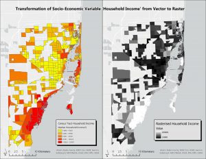
Figure 3. Rasterisation of the variable ‘Household Income’
- Running the Suitability Models:
With all of the factors in usable form, fuzzy membership rules needed to be determined and factors needed to be weighted accordingly before running the suitability models.
3.1 Fuzzy Memberships
Each factor is unique in its impact and spread in terms of vulnerability and risk to sea level rise. Fuzzy memberships require unique lower thresholds, midpoints, upper thresholds and spreads for each variable.
The lower thresholds, midpoints, and upper thresholds for the social variables were chosen by finding the 1st, 2nd and 3rd quartile of each dataset. This meant that there was as little chance of human bias as possible in terms of assigning vulnerability.
For the DEM, two versions were created (one for each RCP scenario), and a scenario range was known for each. The midpoints for the DEMs were chosen by finding the midpoint within the predicted range (ie. if 0.4 to 0.6 meters of expected sea level rise, 0.5 meters as the midpoint), and the upper and lower thresholds were chosen by adding 0.2m of error to the lowest and highest values of the range.
For the distance to coastline, it was recognised that after a short distance from water, the impacts of sea level rise would sharply decrease, leading to the lower threshold, midpoint and upper threshold all being less than 200(m) away from the coast, despite the farthest point from water in the dataset being 18km.
The fuzzy memberships used for each variable were chosen based on the ascertained points, with the membership whose shape best suited the data in question selected. The lower and upper thresholds, midpoints and spread, along with the fuzzy memberships for each variable can be seen in the table below:
Table 1. Fuzzy membership parameters
| Elevation (RCP 2.6) | Elevation (RCP 8.5) | Distance from Coast | % Non-White | Median Household Income | Total Housing Units | |
| Lower Threshold | 0.2 | 0.5 | 5 | 6.395 | 36799.75 | 1433 |
| Midpoint | 0.5 | 0.95 | 100 | 12.65 | 52669 | 1855 |
| Upper Threshold | 0.8 | 1.4 | 200 | 32.095 | 73578.25 | 2396 |
| Spread | 10 | 10 | 5 | 6 | 10 | 5 |
| Fuzzy Membership | Small | Small | Small | Large | Small | Large |
Ultimately, it was decided that it was necessary to create four suitability models, of which two would be devoted to the mitigated scenario, and two to the unmitigated scenario. Within each pair, one would put greater weight upon the physical variables, and one would put greater weight on the socio-economic variables.
The weights assigned to each variable in each suitability model can be seen below:
Table 2. Model of mitigated scenario with weight on physical factors
| Factor | Weight (%) – totalling 100 |
| Elevation | 30 |
| Distance to Coastline | 30 |
| % Non-White | 13.3 |
| Median Household Income | 13.3 |
| Total Housing Units | 13.4 |
Table 2. Model of unmitigated scenario with weight on physical factors
| Factor | Weight (%) – totalling 100 |
| Elevation | 20 |
| Distance to Coastline | 20 |
| % Non-White | 20 |
| Median Household Income | 20 |
| Total Housing Units | 20 |
Table 4. Model of mitigated scenario with weight on socio-economic factors
| Factor | Weight (%) – totalling 100 |
| Elevation | 30 |
| Distance to Coastline | 30 |
| % Non-White | 13.3 |
| Median Household Income | 13.3 |
| Total Housing Units | 13.4 |
Table 5. Model of unmitigated scenario with weight on socio-economic factors
| Factor | Weight (%) – totalling 100 |
| Elevation | 20 |
| Distance to Coastline | 20 |
| % Non-White | 20 |
| Median Household Income | 20 |
| Total Housing Units | 20 |
The purpose of creating four such models was to create a visual sensitivity analysis, in order to see whether there is a significant difference between scenarios, and to understand whether focusing weight on different types of variables would create significant differences in the census tracts affected.
Sensitivity Analysis
The benefit of creating four suitability models within the same mapped area and with the same variables is that a sensitivity analysis was easily conducted as a conclusive understanding of the variety of impact that the variables of different weights gave the model results. A sensitivity analysis is the study of how the variation in the output of a model can be assigned to different sources of variation in the model – they help measure changes in model output when the input variables are manipulated, as was done with the varying DEM ranges of expected sea level rise, and the changing weights for the models. Given the nature of the overall analysis, it was possible to conduct a visual sensitivity analysis, comparing the outputs of the models side-by side to find patterns in the amount of change identified between the models.