fig. 5 wind speed raster
The wind speed that we had obtained was originally a shapefile. However, we are unable to utilize the data if it were a polygon. Thus, we converted it into a raster file (Fig. 5). Similarly, in addition to wind speed, the bathymetry file was also in ASC format, which we were also unable to exploit. We therefore used the conversion tool to transform the file into a raster file.
Based on the Detailed appraisal of the offshore wind industry in China, the limiting distance would be at least 10 km offshore for placing wind turbines. Therefore, we created a buffer zone per the shapefile of China. The buffer distance was 10 km and was then separated into the categories of 10, 20, 30, 40 km from shore, in order to compare results for the Multi-Criteria Analysis, MCE. The limit of 40km was chosen based on current limits in wind farms in China, as most projects are expected to be within 10-40km (Carbon Trust, 2014) (fig. 6)

fig. 6 distance from the shoreline
After obtaining all layers, the next step was to normalize the three layers—bathymetry, wind speed, and distance raster—to a common scale so that we were able to compare them. This was done by using the Reclassify Tool and the Fuzzy Membership Tool, which assigns each raster a value between 0 and 1. For windspeed layer, we implemented the fuzzy membership function through a linear transformation between the user-specified minimum value, a membership of 0, to the user-defined maximum value, which is assigned a membership of 1 (ArcGIS, n.d.).
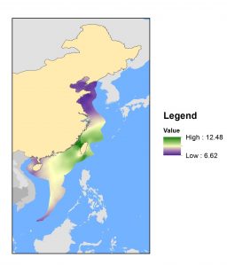
Therefore, for the wind speed raster, we assigned the maximum value as the maximum wind speed value (while 70 m/s is the limit for wind turbines, the maximum was 12.48 m/s) (World Bank, 2008), and a minimum value of 6m/s as studies have found that it is the average wind speed in a particular location to exceed the limit for a small wind turbine to be economically viable (Level, 2017) (Fig.7).
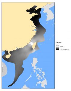
fig. 7 wind speed fuzzy
As for sea depth, our chosen maximum depths were at sea level (0m), we then determined the value of -12m as the minimum based on China’s expectations for installing the majority of wind turbines in the short-to-medium term in water depths no more than 12m (Carbon Trust, 2014). Therefore, we used the reclassify tool to limit the depths of our chosen values (0 for all excluded areas, and 1 for feasible areas) (Fig.8)

fig. 8 classified depth
Finally, for the distance raster, because we had previously applied the buffers, we now merged the buffers and reclassified the values from 10-40km (Fig. 9).
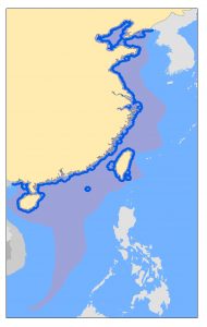
fig. 9 Merged Distance
We now have the three factors normalized and ready for the Multi-Criterion Evaluation (MCE). However, we would still need to determine the weights (relative importance) for each factor. For this step, we utilized an analytical hierarchical approach based on this website. Because we were unable to find information on the relative importance for each layer, we decided that because depth is the largest constraint in establishing wind turbines due to economic factors (Carbon Trust, 2014), it would be slightly more important than the factors of wind speed and distance from shore. Following the same logic based on economic benefits, we decided that wind speed would also be slightly more important than distance from shore, which was based on aesthetic purposes only (Fig. 10).

(Fig. 10) Criteria Preferences
The values after applying relative importance were then calculated (Fig. 11) and rounded to 0.6 for depth, 0.3 for wind speed, and 0.1 for distance to shore:
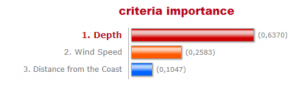
(Fig. 11) Relative Importance Values
The final step is then to overlay the three normalized raster layers by using the Weighted Sum tool based on the numbers obtained from the Analytical Hierarchical Approach (see Results and Constraints section).