Jan 10 – Lecture 1
We’re introduced to the three branches of Landscape Ecology, Health Geography and Crime Analysis. These are the pillars of the course as they form the theme of each assignment and leads heavily into the labs as well.
This introduction class led us to consider three main points for any GIS analysis;
- Where do things happen
- Why do things happen where they happen
- How do things that happen influence other things
- Where should things be located?
Fundamentally, the base principle to GIS needs a location, just as stated in #1. Number 4 considers all the geoprocessing trends to reveal patterns of statistical significance and analyze where a specific event lie in relation to a transcending mean which is effectively a data collection of multiple events.
I got to understand the juxtaposition between Biotic vs Abiotic – Patterns vs Processes. The biotic patterns work in conjunction with the abiotic patterns to allow for the biotic processes and abiotic processes. I can imagine at this point how it would work especially well with landscape ecology, but it should also have implications to health geography as well. There is scope to analyze the biotic patterns and processes by way of spatial analysis of disease spread.
The lecture informs me that GIS is a relationship between human geography – natural environment – natural resources – economic activity. This requires assessing the need of the situation, acquiring the data and the right tools, as well as performing the right method of GIS methodologies. Thinking spatially seems to be the way to go, I can still recall survey modeling for mapping, when we viewed location as the extent and distribution as the pattern to interlacing all the layers together to make a GIS model representation of the real world. The order is entirely subjective to the project but the classic example brought up a few times is the layer of inhabited point shapefiles, along with the road polyline, buildings polygon, hydrological features and land use basemap – when all of it is interlaced and combined, theoretically it should represent what that specific task is looking to model of the real world.
Jan 17 – Lecture 2 Why is geography important
The title of the lecture led me to a little giggle – just first impressions because I am here in this major so it definitely is important and interesting to myself.
I am interested in the Multiscale Analysis within this lecture. It deals with working with study areas – larger to smaller and vice versa – and to see that some relationships that we can decipher an average over an entire study area don’t always apply when viewing it in parts. The example raised in the lecture was a forest within a hydrological system, which starts from pool vegetation – to catchment vegetation – and then to a full river basin. The different patches function differently as influenced by the different microclimate, vegetation cover and slope aspect, which has secondary implications in hortonian/saturated overland flow and the “drainability” of the soil. Greater slope aspects see soils, which are much better drained, albeit there is usually less soil on a greater slope. I take away the scale (spatial domain of study), grain (minimum resolution of data) and extent (scope and domain of data) as very useful concepts from this lecture.
When I got to the Modifiable Aerial Unit Problem point, this has been introduced in 370 and thoroughly went over so I am familiar, yet happy that it’s emphasized as a very important issue, because it is. It is virtually endemic to all spatially aggregated data. The perpetual question pertaining to MAUP is what constitutes a study area? There are infinite possibilities to divide up the data and manipulate it to gain the sort of averaging pattern you want others to see. On a federal level, Gerrymandering takes this concept to heart. The electoral college and district divisions of some cities are astonishing and needlessly complex with the very obvious intention of manipulating voter averages based on past voter patterns of that area. The edge effect is similarly relevant and changes the border relationship between the two entities – we’d like to think of the juxtaposition between smooth/abrupt but there is more to it as well.
New concepts to me from this lecture included Kriging, which is a method of spatial interpolation – scholastic, smooth, abrupt, exact. Not entirely sure if I will get to use it, but another two pertained to spatial autocorrelation, which are the Moran’s and Pearson’s indexes. I have had other methods of spatial autocorrelation before so expecting these to be a variation to spatiality of data.
Jan 24 – Lecture 3 Understanding landscape metrics – patterns and processes
This lecture seems like a precurser to Lab 2. The landscape metrics theory here should tie in well with the lab, especially where we’d be using fragstats – an app with numerous landscape metrics functions.
A contentious issue I faced early on is to qualify the Processes vs Form suggested in the lecture. I’m thinking this is when the issue making maps, where the outcome and objective is to have a finished form in mind, yet the journey itself is a realization of processes. The 3 types of spatial autocorrelation (environmental, biological, unexplained) in here is welcome, yet would be better to have it introduced before all the variables with the Moran’s and Pearson’s of last week.
The map below really interests me. I have been dong a lot of research for fun on the Last Glacial Maximum for a couple of years now and the information keeps on coming. Here we see a map of three types of vegetation reclaiming the land further north as the Laurentide ice sheet retreats and melts into its remnants today as the small ice caps on Baffin, Devon, Ellesmere. You can make the argument that the High Arctic islands had their own ice sheet, separate from the Laurentide, Cordillera or Greenland, but it does not feature as prominently on the research papers as much as the other two which are known to be certain.
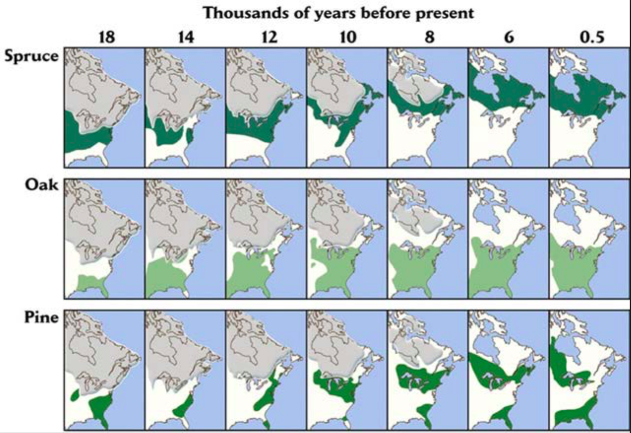
Spruce and Oak is fairly straightforward. You can see that wherever the spruce occupies, Oak will take the adjacent area to the South. The spruce distribution migrated from the Contiguous US to Canada, covering what is now Quebec, Labrador, Ontario and a bit of northern New England. Oak comes to displace Spruce’s glacial maximum range. I’m more curious about the pine as it occupies both, and breaks into two remnants as you can see on the map. Pine is a known boreal rest species so its presence in Ontario is unquestioned, but right there you can observe another colony around Florida and the Southeastern US. What are the implications around the taxon similarities between the two groups? How do we know each has not had speciation adaptation to survive in their respective environments? The Florida pines might be warm-weather pine, like the kind that exists in the North African Mediterranean and along the Canary Islands.
It would be interesting to consider topographical features – as mentioned in the lecture – to this situation. North America is well known for the numerous glacial lakes and other periglacial landforms scattered all over the continent with the departure of the ice sheet. A GIS database on such a phenomenon has major implications in the way we can ease access and provide understanding of landscapes and the geology before we hand the data over to – lets say – an architect or city planner building new structures on previously unused land.
Very interesting example down below on the biotic factors and the animals. It does make a lot of sense to see the difference between a squirrel seeing non-habitat lands as an opportunity, whereas a bear sees it as a threat and consequently avoids such an area. This is something I never thought about and i’m glad to hear it – makes me want to expand more on this area individually.
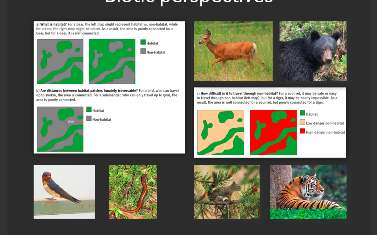
If animals have overlapping ranges and areas to be in or avoid, then the other part of the lecture is just as highly relevant – the fragmentation of forest habitats by human activity. Fragmentation of forests are a staple of human activity if you just take one look at any satellite imagery over a rural area where farmlands are organized and forests cut down into blocks of squares scattered over the landscape. I would want to see whether GIS can map all of the ‘disturbances’ that human activity throws into an area and divides an animal population. Features like a major highway or an oil pipeline inhibits movement to the other side and will subsequently cause some accidents.
Feb 7 – Lecture 4 Statistics Review
NOIR (Nominal, Ordinal, Interval, Ratio) immediately caught my eye. The concept was prevalent throughout 270 and 370. For Nominal, attributes are only named, therefore the relationship between one to the other can’t necessarily be quantified much. For Ordinal, attributes can be ordered, and for Interval, distance is meaningful. Ratio gives clear information as is self-explanatory. All this requires a population sample, and we are introduced to random and systematic errors, which is a key concept borrowed from statistics but just as applicable here. Random errors are ones without a common source to be traced and ones without a meaningful statistical significance. The results would be dispersed between near the ‘accuracy’ maximum and further away. Systematic errors on the other hand are clustered results, providing consistency and precision, albeit without accuracy. This suggests an inherent error which is providing a static shift of all the results that deviates it from the expected value.
Another statistics application pertains to measures of central tendency and dispersion. It would be easy to just think of the mean, median and mode as classic examples. They still contain the utmost relevance, yet there are new-ish concepts to me from this lecture which deals with the measures of variability, skewness, relative position.
The lecture recommends a quantitative approach to correlations and regressions. This is timely as it also introduces the regression models of Ordinary Least Squares (OLS) and the Geographically-Weighted Regression (GWR). These two will be a feature in labs and a prime geoprocessing method I take away from this course. The OLS is a method for estimating the unknown parameters in a linear regression model, whilst GWR takes the same idea and uses them to model spatially varying relationships. I can see a lot of implications with this to crime analysis already with a minimum of three layers; crime data, population and income. This allows us to see the aggregation of crimes based on the different social classes across one particular city. That is just one example however, so the model can work with a lot more.
Feb 14 – Lecture 5 GIS in Health Geography
This has strong connections to Assignment 2 when Kevin and I took on researching the spatial distribution of hospitals in Costa Rica. In any health geography model, there requires a Host-Environment-Agent relationship. The environment being the parameters for the host of a virus to willingly or unwillingly spread and inflict them on other agents.
I was introduced to the Health model of the Community – Environment – Economy. All of this leads to health geography, the environment sets the parameters for the likelihood of a virus spread and sets out where individuals are spatially aggregated across the environment. Health geography concurrently influences the wellbeing of the economy by proxy of the individuals who inhabit the environment and perform to their optimal max potential with good health, or less than that without. The aspects of environmental justice and socioeconomic factors plays a part in health geography just as much.
Mar 14 – Lecture 6 is Crime Related to Geography
A month since the previous lecture due to all the presentations for GEM 511 students and the midterm break. Crime Analysis – already prevalently introduced in 370 – ties in to Lab 4 and Assignment 3. Sometimes it is talked about so much, I wonder if the original inventors of GIS didn’t at least have some consideration to crime mapping when the formed ESRI and ArcMap.
Crime is a geographical phenomenon and the relationships between an offender’s motives to tackling the location, judge the timing and hinge on the frequency of their acts is clear to see. There are much deeper studies into the psychological motives behind crime attacks that can be studied, yet is beyond the scope of this course or my ability to decipher it within a semester. However, the geographical representation of crimes should at least uncover a few things where offenders plan their way around avoiding surveillance, get in and get out as quickly as possible, and avoid committing crimes in the same area too consecutively. The lecture introduces data clocks and hotspot mapping as some of the numerous methods to achieve this.
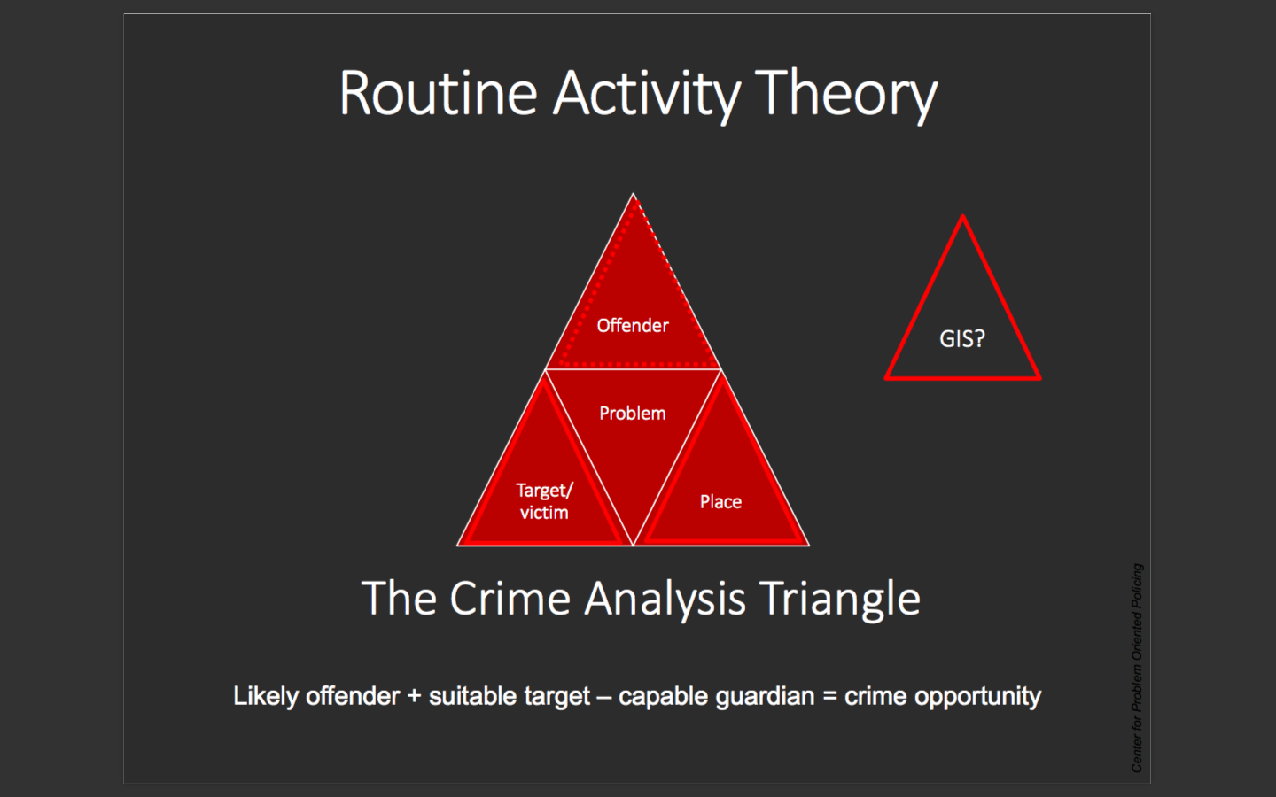
This Routine Activity Theory is new to me and nice to be seen with a visual representation. The relationship between the Offender and victim is certain, and the place varies with each occurrence and type of crime. The place aspect gives rise to geographic profiling and it can do some way to help map crimes. Other, more complicated theories that are also new to me included the rational choice theory and the criminal pattern theory from the lectures. There exists a scope for a lot of extended research I can do in my own time to fully understand it, but from the lectures themselves I could not claim to fully understand them – maybe just the basics.
Mar 21 Lecture 7 – Calgary Crime Analysis
In all honesty I had a fever this week and didn’t attend the lecture per se but was able to fire it up and read through the slides 2-3 days after when I was in sufficiently good condition. Not much to say about this lecture other than that all the information is new to me, and it was wonderful to see how the theoretical processes of crime analysis gets put into practice usage, in this case for Calgary. Fire response teams, protocols, procedures, rules of engagement and the lot is new knowledge and very welcoming. Brian and Chelsey had a conversation that I was next to one time and it was on the response times of these teams. With GIS you can locate the optimum route between the source and destination, set a certain speed and calculate within the margins of error a reasonable time frame in which the response team is expected to show up. These often have discrepancies to actual response times, and is a source of tension and conflict when independent researchers raise up the point.