
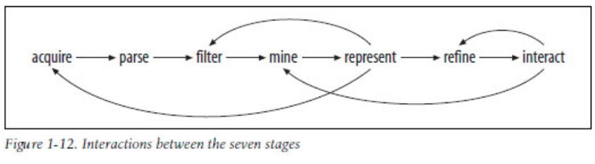
After being introduced to data processing and mapping techniques in R, as well as the theoretical framework of data representation — “data visualization pipeline”; this page details the development of a simple interactive web map using R and its Leaflet library . (main structure of the code provided by TA – Joey K Lee https://github.com/joeyklee/aloha-r, and it’s modified / reflected upon to create this map based on an alternate dataset)
ACQUIRE
Vancouver crime data 2006: http://data.vancouver.ca/datacatalogue/crime-data-details.htm
The Hex Grid data for Vancouver was downloaded from: https://raw.githubusercontent.com/joeyklee/aloha-r/master/data/calls_2014/geo/hgrid_250m.geojson
Initiating R libraries and add data:
#add tools
install.packages("GISTools")
install.packages('rgdal')
install.packages('curl')
install.packages("devtools")
devtools::install_github("corynissen/geocodeHERE")

library(GISTools)
library(rgdal)
library(geocodeHERE)
library(curl)
library(sp)

#acquire
fileName = 'C:/Users/Yuri/Desktop/GEOB_472/data/van_crime_2006.csv'
crime_2006 = read.csv(fileName, header = T)
print(head(data))
*data was downloaded for 2003 – 2015, data for years other than 2006 was deleted in Excel Spreedsheet.And was then read in to R.
PARSE
Parsing is:
- analyzing the characters / strings of symbols to determine the syntactic relation of them and their conformity to formal language rules
- Subsequent transformations that may convert data to a different data type, or create column copies with different data types.
Using R to further parse data:
Since it can be seen that some digits of the street address are replaced by “XX” in the column ‘HUNDRED_BLOCK’, the “gsub” function can be used to replace them to 00 to form a valid address to be geocoded.
##CHANGE X TO 0 - remove the X's in location
crime_2006$h_block = gsub("XX", "00", crime_2006$HUNDRED_BLOCK)
crime_2006$h_block = gsub("X", "0", crime_2006$HUNDRED_BLOCK)
##create full address / location for pop up
crime_2006$full_address = paste(crime_2006$h_block,
                                paste(crime_2006$Street_Name,
                                      "Vancouver, BC, Canada",
                                      sep=", "),
                                sep=" ")
crime_2006$popup_location = gsub(", Vancouver, BC, Canada", " ", crime_2006$full_address)
Next the data need to be geocoded in order to have latitude and longitude for mapping. The function prepared by TA Andras take the street, format it, and then creating a “call URL” containing the address to BC government’s geocoding API to get lat and lon coordinates for each address.
#geocode
##define function for geocode
### a function taking a full address string, formatting it, and making
###a call to the BC government's geocoding API
bc_geocode = function(search){
  # return a warning message if input is not a character string
  if(!is.character(search)){stop("'search' must be a character string")}

  # formatting characters that need to be escaped in the URL, ie:
  # substituting spaces ' ' for '%20'.
  search = RCurl::curlEscape(search)

  # first portion of the API call URL
  base_url = "http://apps.gov.bc.ca/pub/geocoder/addresses.json?addressString="

  # constant end of the API call URL
  url_tail = "&locationDescriptor=any&maxResults=1&interpolation=adaptive&echo=true&setBack=0&outputSRS=4326&minScore=1&provinceCode=BC"

  # combining the URL segments into one string
  final_url = paste0(base_url, search, url_tail)

  # making the call to the geocoding API by getting the response from the URL
  response = RCurl::getURL(final_url)

  # parsing the JSON response into an R list
  response_parsed = RJSONIO::fromJSON(response)

  # if there are coordinates in the response, assign them to `geocoords`
  if(length(response_parsed$features[[1]]$geometry[[3]]) > 0){
    geocoords = list(lon = response_parsed$features[[1]]$geometry[[3]][1],
                     lat = response_parsed$features[[1]]$geometry[[3]][2])
  }else{
    geocoords = NA
  }

  # returns the `geocoords` object
  return(geocoords)
}
##geocoding
# Geocode the events - we use the BC Government's geocoding API
# Create an empty vector for lat and lon coordinates
lat = c()
lon = c()

# loop through the addresses
for(i in 1:length(crime_2006$full_address)){
  # store the address at index "i" as a character
  address = crime_2006$full_address[i]
  # append the latitude of the geocoded address to the lat vector
  lat = c(lat, bc_geocode(address)$lat)
  # append the longitude of the geocoded address to the lon vector
  lon = c(lon, bc_geocode(address)$lon)
  # at each iteration through the loop, print the coordinates - takes about 20 min.
  print(paste("#", i, ", ", lat[i], lon[i], sep = ","))
}

# add the lat lon coordinates to the dataframe
crime_2006$lat = lat
crime_2006$lon = lon
It took about 4 hours to geocode 48257 entries. So we want to save the new csv file containing the coordinates to avoid doing it again.
# write file out

ofile = "C:/Users/Yuri/Desktop/GEOB_472/data/geocodedcrime.csv"
write.csv(crime_2006, ofile)

fileName = "C:/Users/Yuri/Desktop/GEOB_472/data/geocodedcrime.csv"
data = read.csv(fileName, header = T)
Final step of parsing: due to the original “XX”s in ‘HUNDRED_BLOCK’, many crime locations contain the identical lat/long. The coordinates of these locations can be offset slightly and the result will be a cluster of points around a certain determined location – avoiding points overlap in the final mapping process.
# --- handle overlapping points --- #
# Set offset for points in same location:
data$lat_offset = data$lat
data$lon_offset = data$lon
# Run loop - if value overlaps, offset it by a random number
for(i in 1:length(data$lat)){
  if ( (data$lat_offset[i] %in% data$lat_offset) && (data$lon_offset[i] %in% data$lon_offset)){
    data$lat_offset[i] = data$lat_offset[i] + runif(1, 0.0001, 0.0005)
    data$lon_offset[i] = data$lon_offset[i] + runif(1, 0.0001, 0.0005)
  }
}
FILTER
The spatial extent of the analysis should be only City of Vancouver. Thus, geocoded entries should be filtered and outlying points should be eliminated.
# ---------------------------- Filter ------------------------------ #
#subset data within bound
data_filter = subset(data, (lat <= 49.313162) & (lat >= 49.199554) &
                       (lon <= -123.019028) & (lon >= -123.271371) & is.na(lon) == FALSE )

#save save save
ofile_filtered = 'C:/Users/Yuri/Desktop/GEOB_472/data/filteredcrime.csv'
write.csv(data_filter, ofile_filtered)
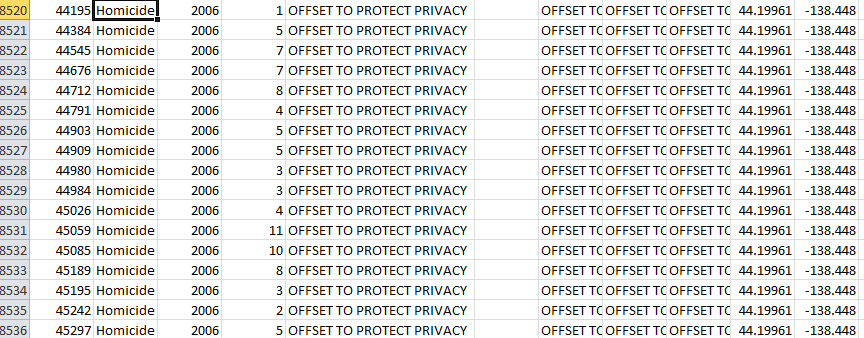
!during my coding process, an error occurred in the represent stage using leaflet when making points layers for each type of crimes; crime type “Homicide” and “Offense against a person” can’t be shown in the points layer even if the layer list is made correctly. Upon inspection back on the entire coding process, the origin of the “error” is found due to the filter process. Since addresses for “Homicide” and “Offense against a person” are in fact obscured in original data (“offset to protect personal identity”), they were given out-of-bound coordinates during geocoding and were essentially filtered out of the dataset during the following process. They thus contain 0 values and can’t be added to the map layers later on.
Instead of being an error on the mapping process, it’s more of a data availability issue – spatial data of the crimes weren’t made publicly available due to privacy protection issues.
After filter the data with year 2006 which I was assigned to, there were 48257 records left. After geocoding, no records were lost. After filtering within Vancouver bound, only 39418 records left. The record lost is due to:
- Address offset of two crime types to protect personal identity
- BC Geocoding API weren’t able to locate certain addresses that were reported / generated by substituting “xx” to “00”.
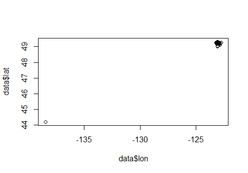
In the above graph, lost record are represent with a dot at the bottom left. The dot contains an overlapping of ~10,000 records that were assigned an unified coordinates out-of-bound.
MINE
Creating Categories / Classification
Categories can be made to tease out some categories to make the data more intuitive for grasping in a map. The first thing is to see what are the types of unique cases that are being called:
# --------MINE--------------------
#examine how the cases are grouped
unique(data$TYPE)
Predetermined crime types were:
- Break and Enter Commercial
- Offense Against a Person
- Other Theft
- Theft from Vehicle
- Break and Enter Residential/Other Mischief
- Theft of Vehicle
- Homicide
Since Homicide and Offense Against a Person are essentially void categories, rest of the types were grouped into 4 categories for representation. They were put into vectors, and a “cid” so that it would easier to identify and represent them later:
# Determine categories to group case types:
Break_and_Enter= c('Break and Enter Commercial','Break and Enter Residential/Other')
Theft_Vehicle_Related= c('Theft from Vehicle','Theft of Vehicle')
Mischief = c('Mischief')
\Theft = c('Other Theft')

#Assigning Categories a Unique Id (CID)
data$cid = 9999
for(i in 1:length(data$Case_Type)){
if(data$Case_Type[i] %in% Break_and_Enter){
data$cid[i] = 1
}else if(data$Case_Type[i] %in% Theft_Vehicle_Related){
data$cid[i] = 2
}else if(data$Case_Type[i] %in% Mischief){
data$cid[i] = 3
}else if(data$Case_Type[i] %in% Other_Theft){
data$cid[i] = 4
}else{
data$cid[i] = 0
}
}

print(unique(data$cid))
The print shows 1,2,3,4,0, so all good!
To answer insight questions:
#--insights: top crimes?
top_crimes = data.frame(table(data$Case_Type))
top_crimes = top_crimes[order(top_crimes$Freq),]
print(top_crimes)
# answer = Other Theft and vehicle theft over 10,000 entries
Save filtered data and create Shapefile / Geojson
- -define the projection type of the shapefile (WGS84)
- -define a folder where the files we create are stored
- -write files out
#save save save
ofile_filtered = 'C:/Users/Yuri/Desktop/GEOB_472/data/filteredcrime.csv'
write.csv(data_filter, ofile_filtered)

#-------create shapefile and Geojson----------------
# --- Convert Data to Shapefile --- #
# store coordinates in dataframe
#CREATE COORDINATES IN WGS84

coords_crime = data.frame(data_filter$lon_offset, data_filter$lat_offset)
# create spatialPointsDataFrame)

data_shp = SpatialPointsDataFrame(coords_crime, data = data_filter)
# set the projection to wgs84
projection_wgs84 = CRS("+proj=longlat +datum=WGS84")
proj4string(data_shp) = projection_wgs84
#OUTPUT FOR .shp FILES and .geojson
geofolder = 'C:/Users/Yuri/Desktop/GEOB_472/data/'
# Join the folderpath to each file name:
opoints_shp = paste(geofolder, "crimes_", "2006", ".shp", sep = "")
print(opoints_shp) # print this out to see where your file will go & what it will be called
opoints_geojson = paste(geofolder, "crimes_", "2006", ".geojson", sep = "")
print(opoints_geojson) # print this out to see where your file will go & what it will be called

# write the file to a shp
writeOGR(check_exists = FALSE, data_shp, opoints_shp, layer="data_shp", driver="ESRI Shapefile")
# write file to geojson
writeOGR(check_exists = FALSE, data_shp, opoints_geojson, layer="data_shp", driver="GeoJSON")
Represent
After data processing, it’s time to represent them in a visual form – map using leaflet tool in R. Adding leaflet library and initiating map.
#working with visualization - representing data in a map using leaflet
#write file in

filename = "C:/Users/Yuri/Desktop/GEOB_472/data/filteredcrime.csv"
data_filter = read.csv(filename, header = TRUE)


# install the leaflet library
devtools::install_github("rstudio/leaflet")

## add the leaflet library to script
library(leaflet)

# initiate leaflet
m = leaflet()
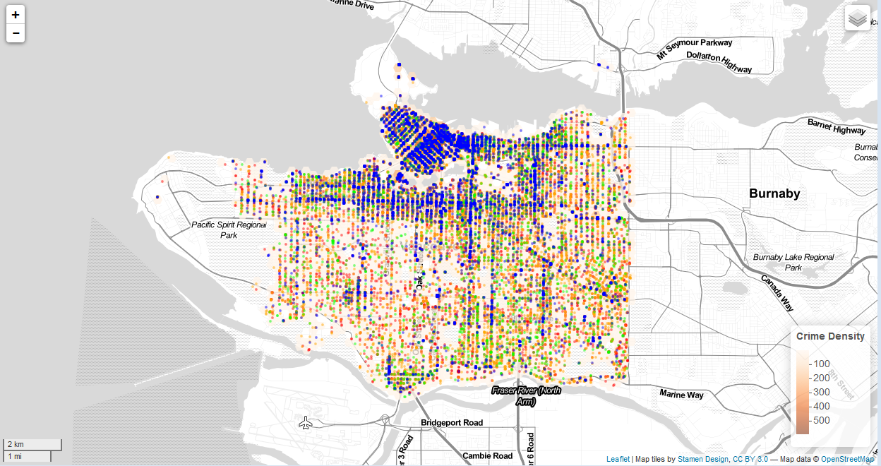
Then leaflet use tiles to form the basemap, default option is to add open street map, other base layer can also be added such as “Stamen toner” which provides a clear grey n white visual.
Adding Polygon Layer with Crime Counts
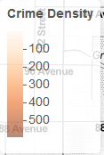
Then the hexgrid generated by Joey should be added as a layer, with shades of color being assigned to hexagons containing different number of crimes. Colorbrewer can generate colors – Oranges are used in this case to illustrate the “hot spots”, domain of the gradient is ‘hexgrid_wgs84$data’.
Corresponding legend is then added to the map.
# add tiles
m = addTiles(m, group = "Open Street Map")
m = addProviderTiles(m,"Stamen.Toner", group = "Toner")

library(RColorBrewer)

#write in hexigons
pal = colorNumeric(
  palette = "Oranges",
  domain = hexgrid_wgs84$data
)

m = addPolygons(m,
                data = hexgrid_wgs84,
                stroke = FALSE,
                smoothFactor = 0.1,
                fillOpacity = 0.8,
                color = ~pal(hexgrid_wgs84$data),
                popup= paste("Number of Crimes: ",hexgrid_wgs84$data, sep=""),
                group = "hex"

# add legend
m = addLegend(m, "bottomright", pal = pal, values = hexgrid_wgs84$data,
              title = "Crime Density",
              labFormat = labelFormat(prefix = " "),
              opacity = 0.55
)
Constraint:
The choropleth map for the hexagon grid seem to be made using “equal interval” method, there isn’t an easy way to change the classification to “natural break” or quantile method. When using equal interval, a lot of areas (hexagons) containing less than 50 cases of crime are shown in a very light color gradient close to white and can hardly be seen.
Adding Points Layer Representing Each Crimes
The subset() function can be used to store data into separate variables, and assign cid to unique variables, so that they can be looped through and different point markers can be added to each category of values – different colors represent different crime type, one points for one incidence.
#add colored points

# subset out , put those variables into a **list** so we can loop through them

data_filterlist = list(df_Break_and_Enter= subset(data_filter, cid == 1),
                       df_Theft_Vehicle_Related = subset(data_filter, cid == 2),
                       df_Mischief = subset(data_filter, cid == 3),
                       df_Theft = subset(data_filter,cid ==4)
)

#variable list
layerlist = c("1 - Break_and_Enter", "2 - Theft_Vehicle_Related",
              "3 - Mischief","4 - Theft")

colorFactors = colorFactor(c('red', 'orange', 'green', 'blue'), domain=data_filter$cid)
for (i in 1:length(data_filterlist)){
  m = addCircleMarkers(m,
                       lng=data_filterlist[[i]]$lon_offset, lat=data_filterlist[[i]]$lat_offset,
                       popup = data_filterlist[[i]]$Case_Type,
                       radius= 2,
                       stroke = FALSE,
                       fillOpacity = 0.5,
                       color = colorFactors(data_filterlist[[i]]$cid),
                       group = layerlist[i]
  )
}
Layers control can then be generated, this allows users to utilize the interactive features of the map without getting overwhelmed by hexagons and points displaying all at once which may become visual noises for map readers.
We want:
- Different base layers that can be pulled out / switched upon depending on users’ preference.
- Categories of individual crimes overlaid on the basemap for users to see crime occurrence.
- Hexagon grids which contains crime distribution (hot spots) in each areas. Hexagon grid should also be a layer that can be individually displayed, otherwise due to most hexagons having a light shade of color, they are obscured by points.
Lastly a scale is added since map will be zoomed in and out, it would be good to have a scale reference.
m = addLayersControl(m,
                     baseGroups = c("Toner Lite",'Open Street Map'),
                     overlayGroups = c("1 - Break_and_Enter", "2 - Theft_Vehicle_Related",
                                       "3 - Mischief","4 - Theft","hex")
)


m = addScaleBar(m,
                position = "bottomleft",
                options = scaleBarOptions()
)
Discussions:
Limitations and Errors:
File Type
Geojson is a file format encoding a variety of geographic data structures, along with their attributes. It contains all information in one file, and can be opened in an editor and make changes. It’s most useful when working with programming languages.
Shapefile is a geospatial vector data format for use in GIS. The format actually involves multiple files that hold the data required for a single map. Shapefile contain more data types and also styling information, so we can use them in ArcGIS to make maps and export to Adobe Illustrator / image to style.
XLS is the main binary file format for excel spreadsheet. It holds information of content and formatting. If I want to make charts, graphs, or do conditional formatting using Excel, then I would want to use xls format since they can be saved in this format.
Comma-Separated Values files hold plain text as a series of values (cells) separated by commas (,) in lines. These file can be opened in editor for reading and editing. If I want to use programming languages to read a spreadsheet and make changes to it, I would use csv format.
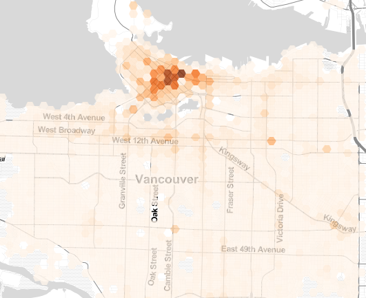
The Final Map
Crime is concentrated in downtown middle and east side with high counts from 200-500+, false creek region display moderately high crime rates, with areas of 100-200 cases. Rest of the area (also most of area) contain low counts from 0 – 50. Theft and theft from vehicles are the most prominent form of crime with 10,000+ incidents, and have a wide distribution throughout the city.
Other data such as population and areal scope other than hexigon grids (neighbourhood / Dissemination area) would be useful to add to mapping. These factors can be normalizing factors to represent spatial distribution of crime from alternative perspectives and may be of more use to the public to know their neighbourhoods.
Interactive features are useful. In static map, each areal units can’t be zoomed and read closely, while in interactive map each grid can be inspected closely, overall distribution and individual occurrence can be shown spontaneously . It can give viewers a better sense of crimes in city, in their neighbourhood or neighbourhood of concern.
And through layer control, types of crime can be added / deleted to the map, thus integrating all data at once and also minimize visual noises, allowing users to grasp crime distribution in types, and make comparisons based on the toggle-able point layer design.
Proprietary software like ArcGIS and Illustrator have extensive capabilities in representing data intuitively based on pre-designed point-and-click functions. They are more “user-friendly” in a way that user only need to know what the tools do and what outcomes can be expected. They are also very matured and well-developed software that has their specialities. For example, ArcGIS has advanced analytical features that can be used in environmental consulting, and Illustrator’s drawing abilities etc. Although they are expensive and aren’t useful in interactive web design, their strong capabilities in their respective field still establish them as very powerful tools
FOSS are much more useful in creating web-based interactive maps since most of them are based on certain programming languages and can be easily exported to html. R has high level programming abilities, with a few lines of code, data processing and plotting can be achieved. All kinds of “plug-ins” – libraries can be added to R to achieve specialized goals. It can be seen that geocoding, plotting, and visualization can all be achieved in R using packages and codes. It also has the potential to make the process semi-automated to create visualization framework to process different data if needed. FOSS also boasts a large and wide user community, which enables learning and sharing among users and develop the platform’s utility along the process.