Methods of Spatial Analysis

With data acquired and generated in previous section, spatial data processing, value extrapolation and route analysis are then completed in ArcGIS.

Data Filtering 

Several steps was taken to further parse / filter data: 

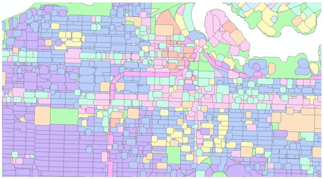
1. Land use was obtained for entire GVRD region –> “select by feature” tool to keep land use polygons with specific spatial attribute–> Region: UBC, UEL (university endowment land), Vancouver –> new layer 
2. Clipped the obtained BC major-road data to the scope of Vancouver city boundary
3. Changed projection of roads
4. Clipped the city intersection data which contains every single intersections to only major road intersections. 

(D can be a rather controversial step and can increase the potential error of estimation associated with the analysis. Primarily due to a lack of data on traffic volume and associated analysis on how PM concentration correlates with volume of traffic, combined with the mention in Thai’s study that no clear correlation was found between road type & concentration fluctuation,  this step was made as a simplified substitution to represent traffic emission. It can be justified to some degree since it’s mentioned in various studies that cyclists are exposed to relatively low level of PM compared to other mode of transport because they can bypass traffic, thus it can be inferred that traffic-related exposure cyclists experience mainly occur at congestion / intersections where traffic is side by side with cyclists. As a result ,the intersections on major road are then selected as a generalized representation of traffic-induced increase in exposure.)

Land use concentration was directly entered in attribute table to 10 land use categories by “select by attribute & field calculator” functions .

(land use concentrations

Spatial Analysis

As mentioned previously, traffic and construction induced increase in emission diminishes when moving away from source areas. Thus, it’s crucial to create a “surface of decay zones” to properly quantify the influence.

First thought was use “buffer” tool to create a zone around the source to reflect its distance of impact (1). However, this method can’t reflect the gradual decay of impact as one moving away from the source. While creating buffers around buffer can render a “zonal decay” surface (2), it still couldn’t model the  smoothly diminishing impact that’s prescribed in this case (3).

 

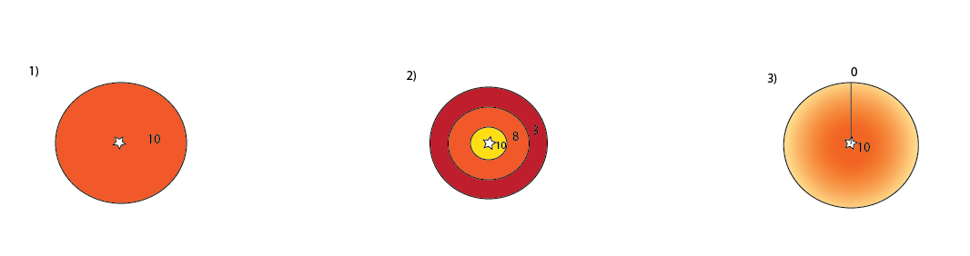
After some  exploration and benefiting from the suggestions made by Jose, it’s been discovered that a combination of tools used in lab exercise can be used to generate a “decay surface”：

Euclidean distance  + fuzzy membership (linear)

(spatial extent)           (reclassify based on membership status of spatial extent)

Euclidean distance tool generate the extent of impact.

The Fuzzy Linear transformation function applies a linear function between the specified minimum and maximum values. Anything below the minimum will be assigned a 0 (definitely not a member) and anything above the maximum a 1 (definitely a member).The spatial extent was assigned as the minimum and 0 m from source assigned as the maximum. A negative linear relationship was then adopted to reflect the decaying “possibility” of a location to be influenced. While the possibility is on a scale of 0-1, it can easily be transformed into concentration value using raster calculator. 

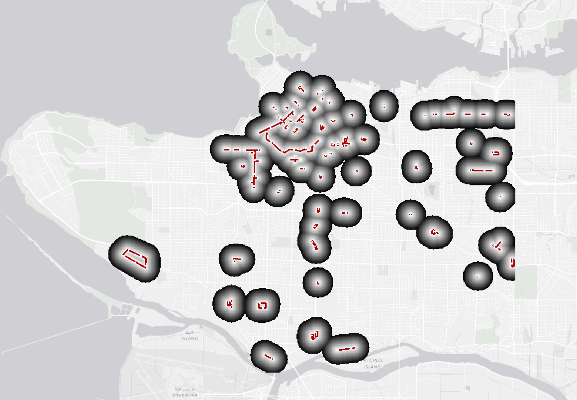
The decay surface for intersections:

The decay surface for construction sites:

 

some trouble shooting processes:

Issue 1:

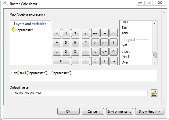
since construction sites and intersections are not continuous surface, there are areas with no data, when using Raster calculator to add values up in raster layers, areas with no data will prevail and the result will render most of the city with null value..

Solution:

– replace the NoData cells in raster layers to a specific value (0 in this case) using a function in raster calculator

Issue 2:

Land use layer doesn’t contain roads, thus the previous problem – areas that contain no data and causing Raster calculator to null values occurs again (since ~half of designated bike ways are on road-right-of way)

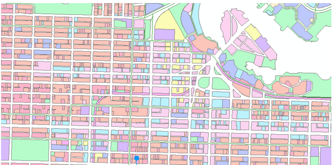land use layer without values for roads that’s causing trouble

 

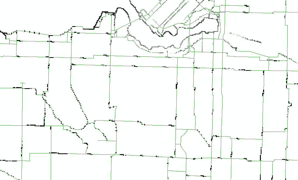
broken lines rendered by the issue (green – entire bikeways; black – bikeways with value assigned)

Solution: buffer around land use polygons to cover the roads in between (20m covers all layers), filling the gaps so the result raster created won’t contain cells with no data.

fattened land use types

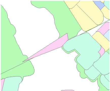
Issue 3: 

Burrard bridge is not included in any layers, while there are designated bikeway on the bridge

Solution:

edit feature to create polygons that works as landuse polygon – and assign its value to 65. *fill other unfilled area. 

 

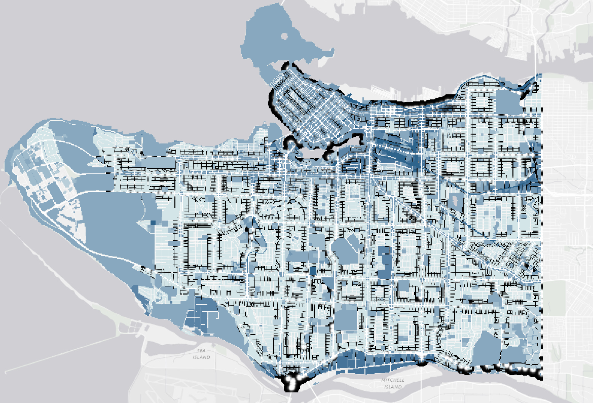
Build concentration surface of the city

compared to using MCE that standardize factors and assign weights to reflect the relative importance of factors, the data created in this project is already in uniformed unit – µg/m^3. A simple sum using raster calculator can construct the city concentration raster surface one-stop:

 

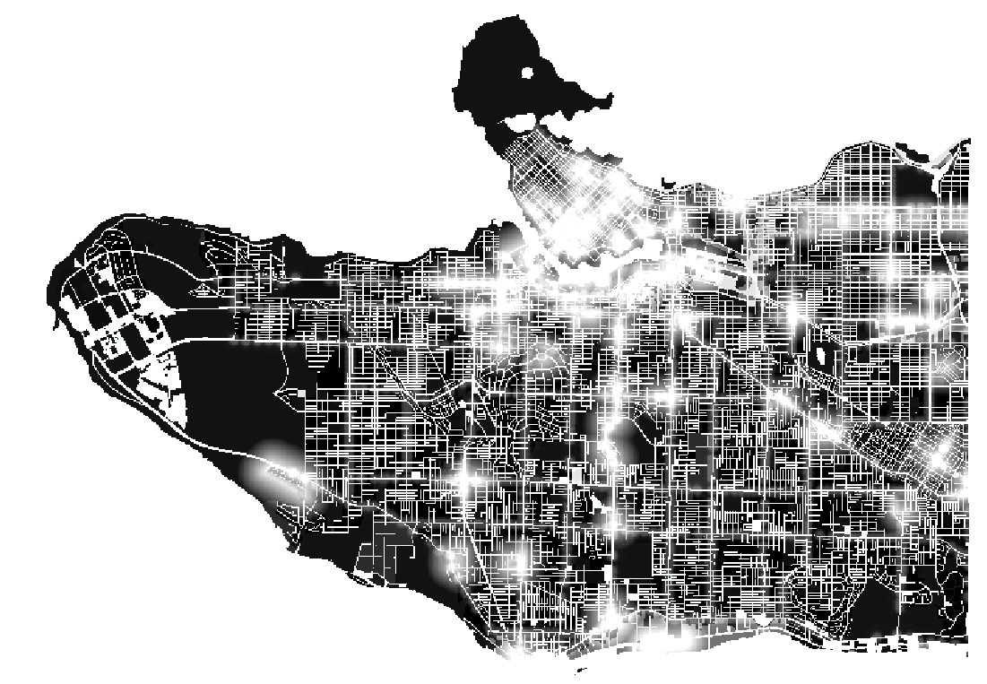
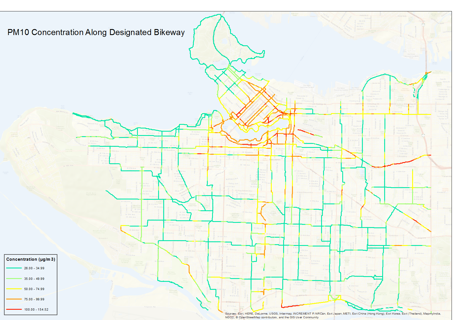
Then the city surface has to be overlaid with designated bikeways layer to gain final results of bikeway values.

Experiment of tools:

1. intersect : only work for geometric extraction
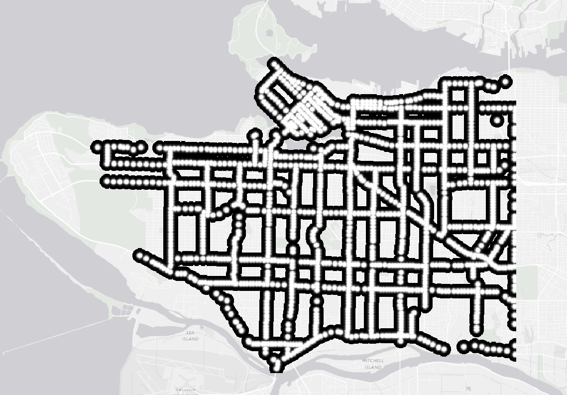
2. run“Feature Vertices to Points” for the bikeway polyline and use sample tool to assign value: not extracting all the cells that constitutes the bikeways

Right tool: extract by mask where the raster layer provides the surface containing value that can be extracted, and the “feature layer” = bikeway polyline as a mask to set the spatial extent of the extraction. 

Final Result:

 

Results & Reflections