Image Processing
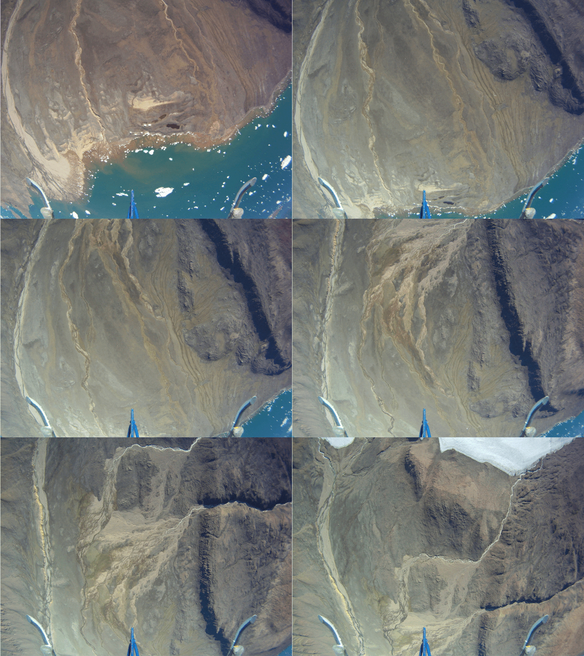
A sample of photos taken of the Alexandra Fiord lowland by a GoPro on a July 2016 helicopter flight.
Introduction
In July 2016, the research team at Alexandra Fiord ran a helicopter flight about 12,000ft above the lowland at Alexandra Fiord and took over 500 air photos. The initial conception for this project was to make use of these photos by using them to create a digital elevation model (DEM) and then making a hydrologic model of the lowland. It became evident that following this path would not be possible, however using the photos to create a 3-dimensional model, a DEM and a orthophoto was still an interesting task that required the application of geographic information science that we learned in this course, and although we didn’t accomplish our final goal, we were able to identify what was necessary in order to create a more robust analysis in future.
Data and Methods
In order to process our subset of 275 air photos (of the over 500 taken,) we used a program called PhotoScanPro. PhotoScanPro aligns the overlapping frames, and creates a three-dimensional point cloud. Prior to frame alignment, we had to calibrate our cameras to account for the fish-eye lens on the GoPro camera. From the point cloud, you then create an overlying mesh, from which you can create a DEM and an orthophoto. At all stages, we chose average quality.
The point cloud and subsequent products can be created in an undefined coordinate system or with the x, y and z dimensions defined by a geographic coordinate system. In order to be properly scaled to the coordinate system there should be several ground control points in the photos being aligned. Although we had a GPS track from our flight, we did not have access to the files that coordinated the times on the GPS and on the GoPro, and therefore, we did not have sufficient reference points when making the model. For our initial point cloud, only three points were identified using landmarks on a pre-existing aerial photo, and as a result our first attempts at the DEM and the orthophoto were not properly georeferenced, and had to be “rubber-sheeted” in ArcGIS, introducing uncertainty and inaccuracies.
Results, Limitations and Error
We did successfully produce a seemingly properly georeferenced orthophoto (See Figure 1.2) after re-running PhotoScan with more accurate coordinates, however the DEM did not seem to be as successful. The east ridge is known to be approximately 700m while the west ridge (“Dome”) is approximately 500m. In the DEM in Figure 1.1, we see that this isn’t the case.
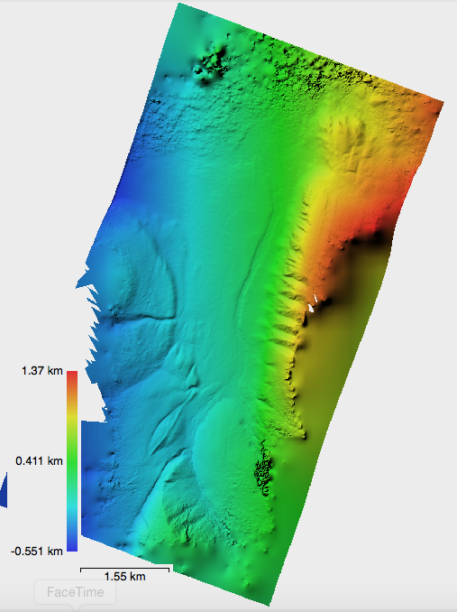
Figure 1.1 Inaccuracies of the AF lowland DEM
We also successfully produced a three-dimensional model (See Figure 1.3) however, we were not able to import it into our GIS due to time constraints. A major limitation in this aspect of the project was that each of these stages took at least 6 hours and in many cases, much longer. The difficulty here was that there was little room for error. However, the level of error was high because this was a learning process.
A few of the sources of error:
• Camera calibration – uncertainty in the level of error
• “Rubber-sheeting” of the improperly georeferenced DEM and orthophoto
• Lower quality settings
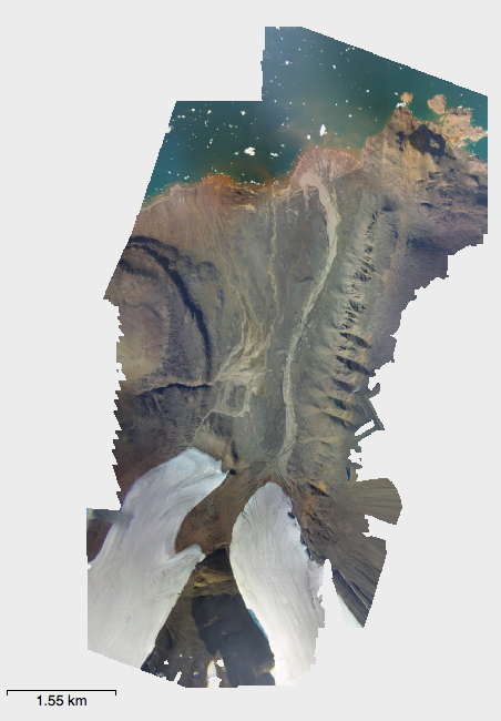
Figure 1.2 Orthophoto compiled from July 2016 air photos.
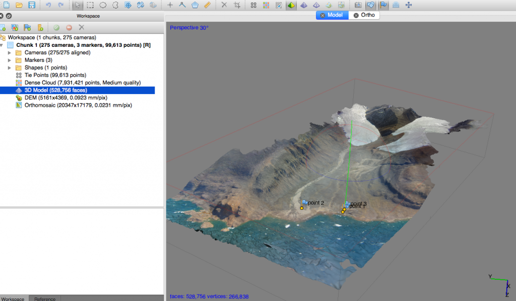
Figure 1.3 A screen capture of the PhotoScanPro workspace, displaying the 3D model created from our dense point cloud.
Further Analysis
Many analyses would open up in this project with the creation of a functional DEM. Many of the parameters we wanted to explore in relation to plant communities depended on an accurate elevation model, including hydrology, solar insolation, slope and aspect.
Additionally, with an accurate, updated orthophoto, as in Figure 1.4, one could create an updated plant community raster layerusing ‘Image Classification’ and accurate, observational data from the field.
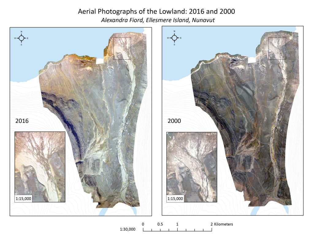
Figure 1.4 A comparison of orthophotos between 2016 and 2000. The photo from 2000 was used to create the plant community raster that we used for our other analyses.
In future, it would be ideal to re-photograph the lowland with this specific GIS analysis in mind. Laying down ground control points, setting up the camera with the GPS and fully grasping the camera calibration would be simple ways to facilitate this process before data collection even begins.