Methods
Plant Communities:
The plant communities that are considered in this project are sedge, dryas, cassiope-vaccinium, and cassiope-dryas. Sand and rock “communities” are also included. The visualization of the plant communities in raster format was produced using aerial and oblique photographs that were taken of the plant communities across the lowland in 2000. They were taken from a helicopter and from the hill east of the lowlands. Using a tool in ArcGIS called ‘Image Classification,‘ an interactive supervised learning tool, the pixels in the aerial photos were classified by colour distribution that were confirmed to be associated with a particular plant community type based on field observations. This was then projected across the lowland to produce the full raster, divided into different community types. In order to complete our various analyses, these had to be converted from raster to vector polygons. We also wanted to simplify the polygons and did so using ‘Focal Statistics’ in ArcGIS, a tool used to perform statistics operations on defined neighbourhoods. We used the majority statistic to determine the most frequently occurring cell (ie. plant community) in our defined neighbourhood, thereby giving us a smoother grouping of plant communities (See Figure 2.1). We used the following parameters to transform our plant community raster:
1. Focal Statistics
in_raster = 2000 plant community raster
neighborhood = rectangle
cell height = 20
statistics_type = majority
output = plantcomms_foc20
2. Focal Statistics
in_raster = plantcomms_foc20
neighborhood = rectangle
cell height = 20
statistics_type = majority
output = plantcomms_foc_double20
3. Focal Statistics
in_raster =plantcomms_foc_double20
neighborhood = rectangle
cell height = 50
statistics_type = majority
output = plantcomms_foc_final
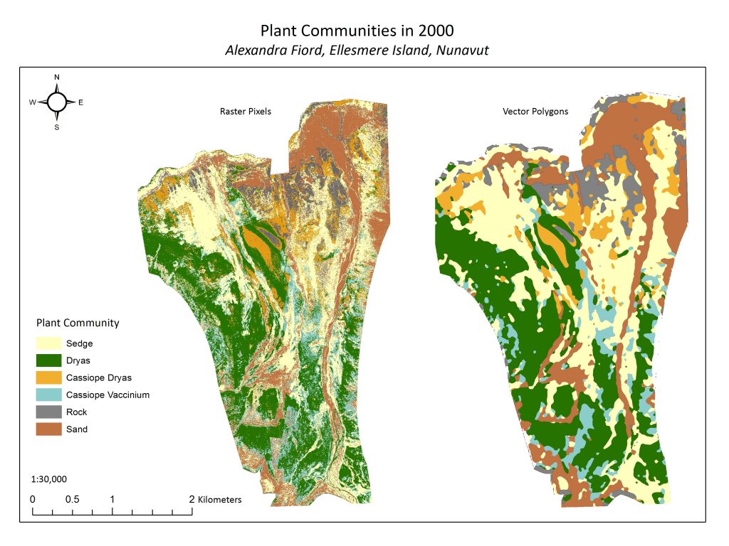
Figure 2.1 A side-by-side comparison of before (left) and after (right) our focal statistics operation and feature class conversion.
We then isolated each community type into its respective raster layers, and then converted each of these layers into a feature class (from Raster toolbox.) Our final products were individual feature classes for each community type.
Temperature
Climate data have been recorded at Alexandra Fiord since 1980 at climate stations located at various sites throughout the lowland. These sites record reference air temperature at 2 meters above the ground in 10 minute intervals throughout the year. In year 2000, additional spatial temperatures were measured using Hobo Pro sensors at 27 locations across the lowland and these are the points we used for our temperature analysis. These temperatures were measured at 10cm above the ground and recorded every 10 minutes from day 170 to 224. In 2010, temperatures were measured at similar locations to 2000, but typically 10-50m off the original points from 2000. These were measured in the same manner, at 10cm above the ground, every 10 minutes, from day 170 to 224. In order to provide a more nuanced visual of the temperatures observed, the point data gathered at the various points for each year was interpolated in ArcGIS using the Kriging method (Figure 2.2)
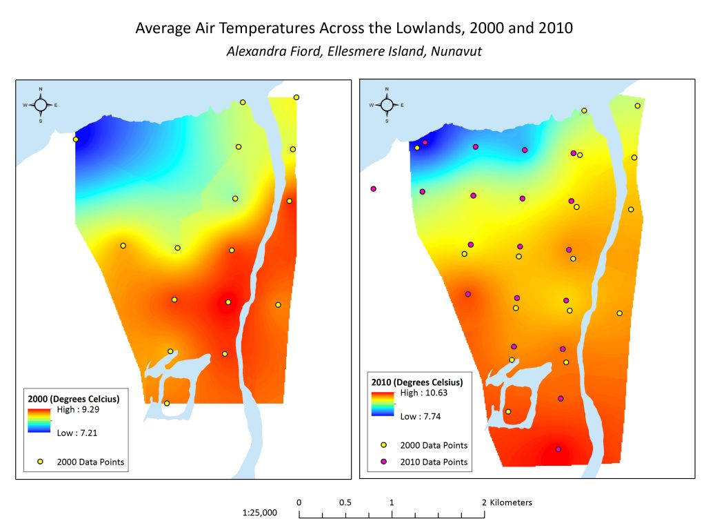
Figure 2.2 Maps showing the interpolated temperature in 2000 and 2010, respectively, with underlying data points. Note that temperature scales are different.
Solar Insolation
Solar insolation was calculated spatially across the lowland using the Accumulated Solar Radiation tool available in ArcGIS. This tool calculates the amount of direct and diffuse solar insolation based on a digital elevation model of the surrounding landscape and the latitude, taking into account the angle and rotation of the sun. The DEM used for this was built in ArcGIS by converting a topographic map of the region into an elevation model, using the topo to raster tool. In the Arctic, solar insolation is unique because there are 24 hours of daylight in the summer and no daylight for a large portion of the year. This was taken into account when inputting the temporal parameters to run the tool. The dates we used were February 10th to November 1st – the days of the year in which there is daylight. By running the tool, solar insolation – based on the shade patterns of the surrounding hills and elevation contours – was predicted across the lowland and averaged out between the selected dates (Figure 2.3).
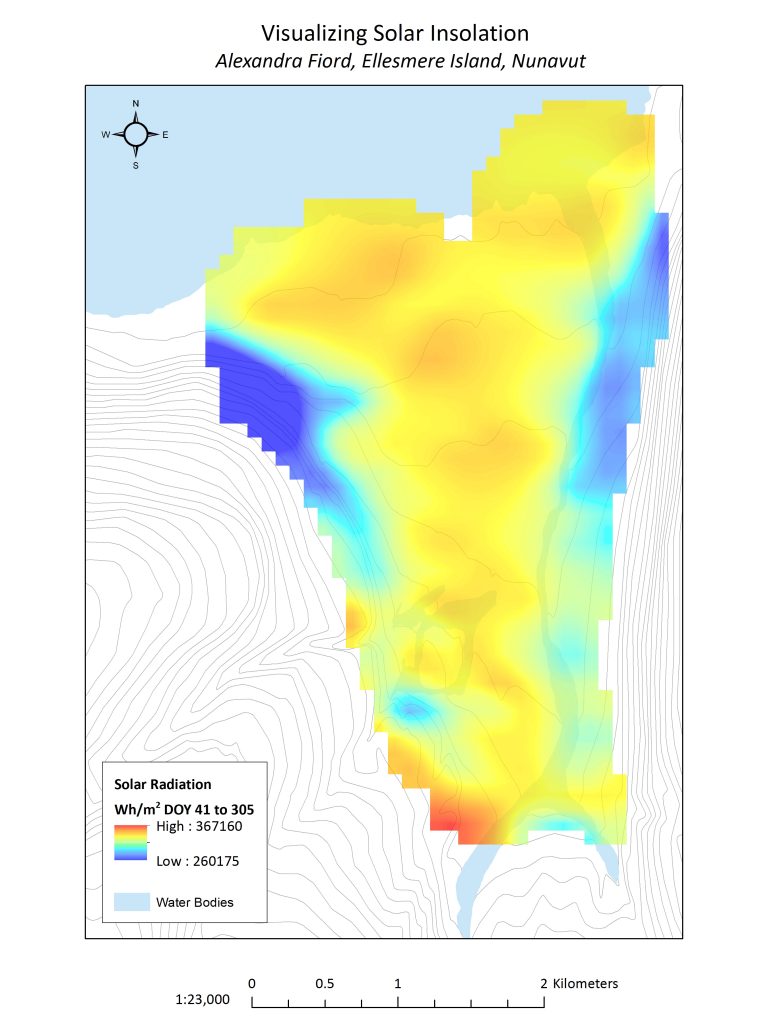
Figure 2.3. Solar insolation at Alexandra Fiord averaged during the typical total insolation period (February 10th – November 1st)
In order to conduct an analysis of how solar insolation might affects the distribution of plant communities, we needed to make some alterations to the community polygons and solar insolation raster. We wanted to test whether some communities have higher levels of solar insolation than others. To do this, we had to create a spatial join between solar insolation data and community polygons. To quantify solar insolation among the polygon data, we converted the raster to point form (Figure 2.4). We found that the solar insolation raster cell size needed to be changed in order to minimize the number of plant communities with a null value of solar insolation due to their relatively small area. After resampling from 100m to 10m and converting the raster to points, we spatially joined each plant community polygon feature to the new solar insolation feature. With joined plant polygons, we could then conduct analyses based on the mean solar insolation and variance per plant community, and test whether there is a statistical difference between them.
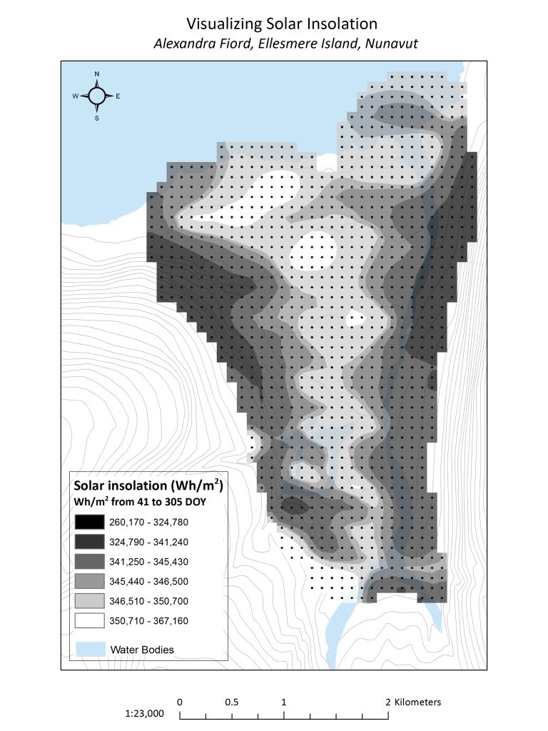
Figure 2.4 Solar insolation map with points representing insolation, which were used to calculate average insolation per plant community.
Snow Melt
The date of snowmelt across the lowland was not recorded spatially in 2000. Instead, aerial photos were taken twice during the period of snowmelt (Day of year (DOY) 160 and DOY 180). These photos were analyzed using the ‘image classification’ toolset in ArcGIS to generate a general map of the snowmelt pattern in 2000. We then compared the percent area of our plant community polygons that remained under snow cover on DOY 160, DOY 180 and then both days, in order to determine which communities were associated with snow cover.