This interactive map of crime in Vancouver was created with the R programming language in RStudio and RLeaflet. As someone who is not proficient in any programming language, it was a difficult experience, but I learned a lot from the process.
######################################################
# Vancouver Crime: Data Processing Script Pt. 1
# Date: 25/10/2016
# By: Jonathan Mak
# Desc: Part 1: Mine and Filter
######################################################

# ------------------------------------------------------------ #
# ---------------------- Install Libraries ------------------- #
# ------------------------------------------------------------ #
# install.packages("GISTools")
# install.packages("RJSONIO")
# install.packages("rgdal")
# install.packages("RCurl")
# install.packages("curl")
# install.packages("leaflet")

# ------------------------------------------------------------ #
# ----------------------- Load Libararies -------------------- #
# ------------------------------------------------------------ #
library(GISTools)
library(RJSONIO)
library(rgdal)
library(RCurl)
library(curl)

# ------------------------------------------------------------ #
# ---------------------------- Acquire ----------------------- #
# ------------------------------------------------------------ #
file_loc <- "/Users/Jonathan/crime_csv_all_years_nolatlong.csv"
data
Install and load necessary libraries, and acquire dataset that has been downloaded.
file_loc is given the location of the file, then the csv is read and written as ‘data’
# ------------------------------------------------- #
# --------------------- Mine ---------------------- #
# ------------------------------------------------- #
# --- Examine the unique cases --- #

unique(data$TYPE)
unique(data$HUNDRED_BLOCK)
unique(data$NEIGHBOURHOOD)
Check the unique cases of different columns of ‘data’ to see what data is needed.
# ------------------------------------------------------------ #
# ---------------------- Filter for year --------------------- #
# ------------------------------------------------------------ #
# Subset only 2010 data
data_2010 = subset(data, (YEAR == 2010) == TRUE )
Subset the original dataset to only include data from 2010. Doing it earlier in the process reduces the time necessary for geocoding the data.
# ------------------------------------------------- #
# -------------- Parse: Geocoder ------------------ #
# ------------------------------------------------- #
# change intersection to 00s
data_2010$h_block = gsub("X", "0", data_2010$HUNDRED_BLOCK)
print(head(data_2010$h_block))

# Join the strings from each column together & add "Vancouver, BC":
data_2010$full_address = paste(data_2010$h_block,
                          paste(data_2010$Street_Name,
                                "Vancouver, BC",
                                sep=", "),
                          sep=" ")

unique(data_2010$full_address)
The data needs to be parsed to be usable. The address data is given in a format that maintains anonymity, so addresses are given with XXs replacing 100 blocks. To make the addresses usable with the BC Government’s geocoding API, these must be replaced with 00s. A new column is created within data_2010 – h_block. The full address is needed, so a new column within data_2010 must be made – full_address, which pastes the h_block with the Street_Name, together with Vancouver, BC.
# a function taking a full address string, formatting it, and making
# a call to the BC government's geocoding API
bc_geocode = function(search){
  # return a warning message if input is not a character string
  if(!is.character(search)){stop("'search' must be a character string")}

  # formatting characters that need to be escaped in the URL, ie:
  # substituting spaces ' ' for '%20'.
  search = RCurl::curlEscape(search)

  # first portion of the API call URL
  base_url = "http://apps.gov.bc.ca/pub/geocoder/addresses.json?addressString="

  # constant end of the API call URL
  url_tail = "&locationDescriptor=any&maxResults=1&interpolation=adaptive&echo=true&setBack=0&outputSRS=4326&minScore=1&provinceCode=BC"

  # combining the URL segments into one string
  final_url = paste0(base_url, search, url_tail)

  # making the call to the geocoding API by getting the response from the URL
  response = RCurl::getURL(final_url)

  # parsing the JSON response into an R list
  response_parsed = RJSONIO::fromJSON(response)

  # if there are coordinates in the response, assign them to `geocoords`
  if(length(response_parsed$features[[1]]$geometry[[3]]) > 0){
    geocoords = list(lon = response_parsed$features[[1]]$geometry[[3]][1],
                     lat = response_parsed$features[[1]]$geometry[[3]][2])
  }else{
    geocoords = NA
  }

  # returns the `geocoords` object
  return(geocoords)
}

# Geocode the events - we use the BC Government's geocoding API
# Create an empty vector for lat and lon coordinates
lat = c()
lon = c()

# loop through the addresses
for(i in 1:length(data_2010$full_address)){
  # store the address at index "i" as a character
  address = data_2010$full_address[i]
  # append the latitude of the geocoded address to the lat vector
  lat = c(lat, bc_geocode(address)$lat)
  # append the longitude of the geocoded address to the lon vector
  lon = c(lon, bc_geocode(address)$lon)
  # at each iteration through the loop, print the coordinates - takes about 20 min.
  print(paste("#", i, ", ", lat[i], lon[i], sep = ","))
}

# add the lat lon coordinates to the dataframe
data_2010$lat = lat
data_2010$lon = lon
Use the BC Government’s Geocoding API to acquire the latitude and longitude of addresses, and write them to data_2010.
# --- handle overlapping points --- #
# Set offset for points in same location:
data_2010$lat_offset = data_2010$lat
data_2010$lon_offset = data_2010$lon

# Run loop - if value overlaps, offset it by a random number
for(i in 1:length(data_2010$lat)){
  if ( (data_2010$lat_offset[i] %in% data_2010$lat_offset) && (data_2010$lon_offset[i] %in% data_2010$lon_offset)){
    data_2010$lat_offset[i] = data_2010$lat_offset[i] + runif(1, 0.0001, 0.0005)
    data_2010$lon_offset[i] = data_2010$lon_offset[i] + runif(1, 0.0001, 0.0005)
  }
}
Many points overlap, so this must be taken into account for visualization purposes, to be able to see the locations of different points. If there are multiple instances of points in the data, it is offset.
# -------------------------------------------------------------- #
# -------------------- Filter pt2 ------------------------------ #
# -------------------------------------------------------------- #
# Subset only the data if the coordinates are within our bounds or if
# it is not a NA
data_filter = subset(data_2010, (lat <= 49.313162) & (lat >= 49.199554) &
(lon <= -123.019028) & (lon >= -123.271371) & is.na(lon) == FALSE )
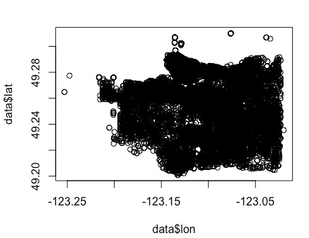
# plot the data
plot(data_filter$lon, data_filter$lat)
ofile_filtered = '/Users/Jonathan/Desktop/GEOB472/Crime/crime-geo-filtered.csv'
write.csv(data_filter, ofile_filtered)
Filter out the data that is not within the bounds of Vancouver. Then, the data can be plotted, and it vaguely forms the shape of Vancouver.
Save the geofiltered data to a file.
*** Part 2: Leaflet ***
First, I load leaflet’s library and access saved data.
# load leaflet
library(leaflet)

#locate data
file_loc <- "/Users/Jonathan/Desktop/GEOB472/Crime/crime-geo-filtered.csv"
data
Then, convert data to a Shapefile and Geojson. It is a multi-step process that requires setting the projection, setting output folder and name.
# --- Convert Data to Shapefile --- #
# store coordinates in dataframe
coords_crime = data.frame(data$lon_offset, data$lat_offset)

# create spatialPointsDataFrame
data_shp = SpatialPointsDataFrame(coords = coords_crime, data = data)

# set the projection to wgs84
projection_wgs84 = CRS("+proj=longlat +datum=WGS84")
proj4string(data_shp) = projection_wgs84

# set an output folder for our geojson files:
geofolder = "/Users/Jonathan/Desktop/GEOB472/CrimeLab/"

# Join the folderpath to each file name:
opoints_shp = paste(geofolder, "crimes", ".shp", sep = "")
print(opoints_shp)
opoints_geojson = paste(geofolder, "crimes", ".geojson", sep = "")
print(opoints_geojson)

# write the file to a shp
writeOGR(data_shp, opoints_shp, layer = "data_shp", driver = "ESRI Shapefile",
         check_exists = FALSE)

# write file to geojson
writeOGR(data_shp, opoints_geojson, layer = "data_shp", driver = "GeoJSON",
         check_exists = FALSE)
After, I acquired joey’s hexagon grid, and read it in. The hexgrid must be transformed to wgs84 to match the point file.
# --- aggregate to a grid --- #
# ref: http://www.inside-r.org/packages/cran/GISTools/docs/poly.counts
# set the file name - combine the shpfolder with the name of the grid
# grid_fn = paste(shpfolder,'hgrid_100m.shp', sep="")
grid_fn = 'https://raw.githubusercontent.com/joeyklee/aloha-r/master/data/calls_2014/geo/hgrid_250m.geojson'

# read in the hex grid setting the projection to utm10n
hexgrid = readOGR(grid_fn, 'OGRGeoJSON')

# transform the projection to wgs84 to match the point file and store
# it to a new variable (see variable: projection_wgs84)
hexgrid_wgs84 = spTransform(hexgrid, projection_wgs84)
I then used the poly.counts() function to count the number of calls within each hexagon grid cell. A data frame is created, and the hexgrid data is set to the dataframe. All grids without any crime occurrences are removed.
# Use the poly.counts() function to count the number of occurences of crimes per grid cell
grid_cnt = poly.counts(data_shp, hexgrid_wgs84)

# create a data frame of the counts
grid_total_counts = data.frame(grid_cnt)

# set grid_total_counts dataframe to the hexgrid data
hexgrid_wgs84$data = grid_total_counts$grid_cnt

# remove all the grids without any crimes
hexgrid_wgs84 = subset(hexgrid_wgs84, grid_cnt > 0)
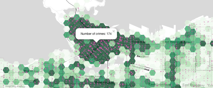
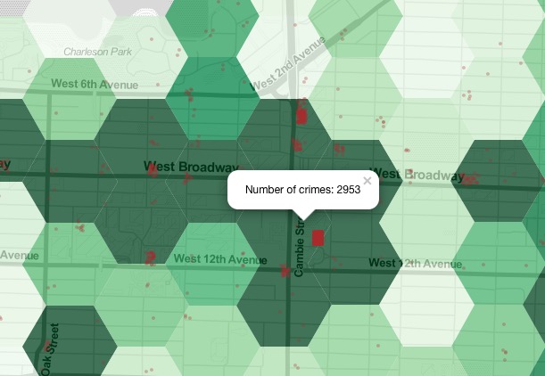
Because the data is highly skewed, the map would have ended up looking like this:
This is because the range of data is from 1 to 2953, with a median of 9 and a mean of 20.85. This data appears erroneous, but I will discuss this later.
To compensate for the error, I set an upper limit of 50 for the data, making the differences in data more visible.
# check data range
summary(hexgrid_wgs84$data)

# set upper limit
hexgrid_wgs84$datalimit
I then wrote the limited hex data to a shapefile and geojson
# define the output names:
ohex_shp = paste(geofolder, "hexgrid_250m_", "crime", "_limited",
                 ".shp", sep = "")
print(ohex_shp)

ohex_geojson = paste(geofolder, "hexgrid_250m_", "crime",
                     "_limited", ".geojson", sep = "")
print(ohex_geojson)

# write the file to a shp
writeOGR(check_exists = FALSE, hexgrid_wgs84, ohex_shp,
         layer = "hexgrid_wgs84", driver = "ESRI Shapefile")

# write file to geojson
writeOGR(check_exists = FALSE, hexgrid_wgs84, ohex_geojson,
         layer = "hexgrid_wgs84", driver = "GeoJSON")
Initiate leaflet and add a more appropriate tile theme
# initiate leaflet map layer
m = leaflet()
m = addProviderTiles(m, "Stamen.TonerLite", group = "Toner Lite")
Then, I needed to store the file nape of the geojson hex grid and read in the data
# --- hex grid --- #
# store the file name of the geojson hex grid
hex_crime_fn = "/Users/Jonathan/Desktop/GEOB472/CrimeLab/hexgrid_250m_crime_limited.geojson"

# read in the data
hex_crime = readOGR(hex_crime_fn, "OGRGeoJSON")
For the limited hex data, a colour palette
# Create a continuous palette function
pal = colorNumeric(
  palette = "Greens",
  domain = hex_crime$datalimit
)
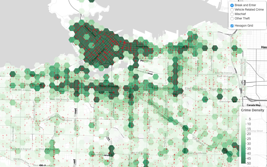
Add hexagon grid to map as polygons, using hex_crime$datalimit
# add hex grid
m = addPolygons(m,
                data = hex_crime,
                stroke = FALSE,
                smoothFactor = 0.2,
                fillOpacity = .75,
                color = ~pal(hex_crime$datalimit),
                popup= paste("Number of crimes: ",hex_crime$data, sep=""),
                group = "Hexagon Grid"
)
# add legend
m = addLegend(m, "bottomright", pal = pal, values = hex_crime$datalimit,
              title = "Crime Density",
              labFormat = labelFormat(prefix = " "),
              opacity = 0.75
)
Subset out your data, ascribe cid
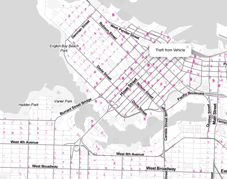
# --- points data --- #

# subset out your data:
df_break_and_enter = subset(data, cid == 1)
df_vehicle_related = subset(data, cid == 2)
# df_homicide = subset(data, cid == 3) ### there are no homicide cases in data
df_mischief = subset(data, cid == 4)
# df_personal_offence= subset(data, cid == 5) ### there is no personal offence cases in data
df_other_theft = subset(data, cid == 6)
There was homicide and personal offence data in the data before filtering out the points outside Vancouver. This may be cases of error, and I will discuss this later.
Next, I put the filtered data into a list to loop through. colorFactors is created to give the point data different colors, and stroke and radius is set to the point data.
data_filterlist = list(df_break_and_enter = subset(data, cid == 1),
                       df_vehicle_related = subset(data, cid == 2),
                       #                      df_homicide = subset(data, cid == 3),
                       df_mischief = subset(data, cid == 4),
                       #                     df_personal_offence = subset(data, cid == 5),
                       df_other_theft = subset(data, cid == 6))

layerlist = c("Break and Enter", "Vehicle Related Crime", "Mischief", "Other Theft")

colorFactors = colorFactor(c('red', 'orange', 'purple', 'blue', 'pink', 'brown'), domain=data$cid)
for (i in 1:length(data_filterlist)){
  m = addCircleMarkers(m,
                       lng=data_filterlist[[i]]$lon_offset, lat=data_filterlist[[i]]$lat_offset,
                       popup=data_filterlist[[i]]$TYPE,
                       radius=2,
                       stroke = FALSE, fillOpacity = 0.3,
                       color = colorFactors(data_filterlist[[i]]$cid),
                       group = layerlist[i]
  )

}
Finally, I add layer controls and show map.
m = addLayersControl(m,
                     overlayGroups = c("Hexagon Grid"),
                     baseGroups = layerlist
)

# show map
m
Process
Loss of records:
Before filtering out the data that wasn’t within Vancouver, it appeared like this:
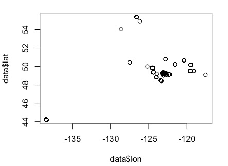
There are many points that lie far outside Vancouver’s boundaries. Before the filtering, there 34286 data points, and after filtering, only 30258 points of data – 12% loss. In addition, all homicide data points (10) and personal offence points (3729) were removed from the dataset, because they had the addresses obscured for privacy reasons. The other removed data points were surely due to some kind of error, either on the part of the data or my own doing.
I also realized that after finishing my map, that while replacing the original addresses (which had replaced 00s with XXs) – that my code to replace the XXs with 00s had replaced all Xs with 0s. Thus, an original address that was ’29XX Expo Avenue’ became ‘2900 E0po Avenue’. This was error on my part.
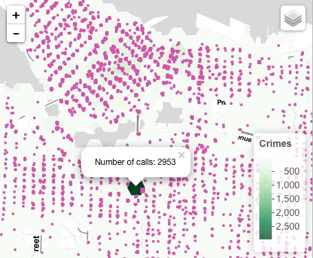
There were also many peculiarities with this data. As I had stated before, there was one area with a massive concentration of crimes reported – the area around Vancouver City Hall, which had 2953 crimes reported. This seems strange and unreliable, as it doesn’t seem to make sense that some areas would have zero crimes reported, and adjacent areas would have thousands reported. I found that using R was complicated in the way that I couldn’t see what the functions were necessarily doing, and not being proficient in the programming language means that it involved a lot of trial and error, but I was unaware of where I was making errors, if I was.
Because of the massive scaling of the data, I had to set an upper limit to the data to make sure it wasn’t scaled disproportionately. However, I did not know how to make the legend display >50 rather than 50 for the highest value.
Working with this data gave me experience with different filetypes. Having worked with ESRI’s proprietary shapefile format before, it was interesting to see it being used in R with code. It was also good to gain experience using geojson files, which are similar to shapefiles but do not have the same amount of data, such as with style information. One would use shapefiles and geojson files for spatial alalysis. Similarly, acquiring data in csv format is useful because it is simply values separated by commas, whereas excel files are proprietary Microsoft files that include information about formatting, style, etc. Creating csv files are useful when doing tabular analysis of data.
Visualization
With respect to cartographic constraints, it was difficult to have full control of the visual aspect of the map because of my lack of experience and knowledge of R and Leaflet. However, Leaflet was simple and intuitive as most of the work as already been done by the person who created the leaflet library.
It seemed interesting, but not unsurprising that most of the crime in Vancouver is centred Downtown and along the Broadway and W 4th corridors. This correlates with population density and the built-up formation of the city, so it is not surprising. I was surprised by the sheer number of break-and-enters within the city.
Reflection
Learning the use of free and open source software has been extremely rewarding for me, because I feel that it is transferrable outside of circumstances that allow me to have access to expensive proprietary software packages. Learning R and leaflet has shown me the things that FOSS is capable of, and the community and documentation that exists for these softwares. However, in many circumstances, the functionality of proprietary software is unparalleled – which is what I find with Adobe Illustrator.
The whole process of doing this project was interesting, but I feel that I couldn’t learn it on a profound level. However, I found the community help of FOSS was good for me in figuring out any problems I encountered.