Methodology

Data Selection:

There were two types of data required for this analysis: Crime data and census data. Crime data was obtained through data.gov in the form of a CSV file. The file contained every crime committed in the city of Chicago from January to August 9th 2018. From armed robbery to illegal betting the file had it all. There were some 240,000 rows of crimes within the Excel file. Using the IUCR codes also obtained from data.gov, I filtered the data to eight specific crimes. These crimes are as follows:

• Homicide first degree (IUCR  110)
• Homicide second degree (IUCR 130)
• Aggravated battery w/ handgun (IUCR 041A)
• Aggravated battery w/ other firearm (IUCR 041b)
• Aggravated criminal sexual assault w/ handgun (IUCR 261)
• Aggravated criminal sexual assault w/ other firearm (IUCR 262)
• Armed robbery w/ handgun (IUCR 031a)
• Armed robbery w/ other firearm (031b)

There are other types of crime which could be considered violent. However, crimes committed with a firearm were my focus due to the increase in shootings. These eight categories totalled 6,223 incidences.

Census data obtained from the United States Census Bureau was delivered in a geodatabase format ready for use in Arcmap. After combing through a very large table describing the alphanumeric codes applied to each type of data I opened both the “Income” and “Employment” tables. The codes were “B19013e1″ for median household income and “B23025e1” for employment status of people 16 years or older. I selected the data in each table and exported both factors including their GEOIDs to a new table for later use. I chose these factors because each has the potential to influence communities. Areas of low income and high unemployment drive people to do things they otherwise may not do in order to make a living. Individually they create a potential for violence in different ways, but they are also related. Often times one tends to exist either in the presence of, or due to the other. 

Preparing Shapefiles for Analysis:

To limit repetitive work I used the model builder in order to clip and project the layers to be used for either analysis or display purposes.

Figure 1 shows the model used to project and clip every shapefile needed. The clip feature used was the Chicago Boundary base map shapefile. The coordinate system used in projection was NAD_1983_StatePlane_Illinois_East_FIPS_1201_Feet. Once the layers were aligned I began joining census and crime data to the census blocks layer. I duplicated the census blocks layer for the purpose of two separate OLS analyses to see which factor (income or employment) had a stronger relationship with crime. Each factor was joined based on GEOID from the table mentioned before to the intended layer. I later created a blocks layer which included both crime and employment data for a third regression. Crime point data were spatially joined to these layers as well.

Ordinary Least Squares Regression (OLS):

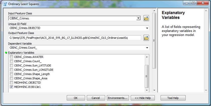
An ordinary least squares (OLS) regression was applied to three layers. These layers were crime vs. income, crime vs. employment, and crime vs. income &  employment. Once I created the layers using spatial and table joins I used the OLS tool under “spatial statistics” in ArcToolbox (Figure 3). OLS shows the spatial relationship between the independent and dependent variables. It is a global linear regression model which creates a line of best fit by squaring the distance from each point in the data cluster to the line (“ArcGIS Pro”). The line is designed to minimize the distance between the points and itself. The process generates an output file displaying detailed results of the analysis which will be discussed in the results section. The output table includes R-squared and T-statistic values. R-squared values fall between zero and one. The larger the value, the more reliable the result. Probability values determine whether or not the model is due to random chance. Values less than 0.05 are considered statistically significant and show the model is not due to random chance but in fact to a relationship between variables. For the purposes of this analysis, every regression will be done with crimes as the dependent variable and either income, employment, or both as the explanatory variable.

Moran’s I:

The Moran’s I tool is used to measure spatial autocorrelation within a data set. Similar to Tober’s first law of geography, spatial autocorrelation is “the degree to which one object is similar to other nearby objects”(“Spatial Autocorrelation”). The output file includes important figures such as the Moran’s I and z-score values. The Moran’s I is a number ranging from -1-0-1. A negative value represents a perfect clustering of dissimilar values (“Moran’s I”). A value of zero represents no autocorrelation or perfect randomness amongst the data (“Moran’s I”). A positive value indicates perfect clustering of similar values (“Moran’s I”). If positive, neighbours are more similar than in randomness. However, clustering of similar values can be high, low, or a mix (“Spatial Autocorrelation”). It does not necessarily mean they are all high values. Pattern analysis tools, such as OLS, generate a “null hypothesis” which essentially “states that there is no pattern; the expected pattern is only of random chance” (“EDN”). Null hypotheses represent spatial randomness meaning values at one location do not depend on values at neighbouring locations (“Spatial Autocorrelation”). The z-score value indicates the likelihood clustered patterns are due to random chance. It is a “test of statistical significance that helps you decide whether or not to reject the null hypothesis” (“EDN”). A high or low z-score exists within the tails of a bell curve related to your data and indicates “it is very unlikely the observed pattern is some version of the theoretical spatial patterns represented by the null hypothesis” (“EDN”). This tool was applied to all three OLS analyses.

Geographically Weighted Regression:

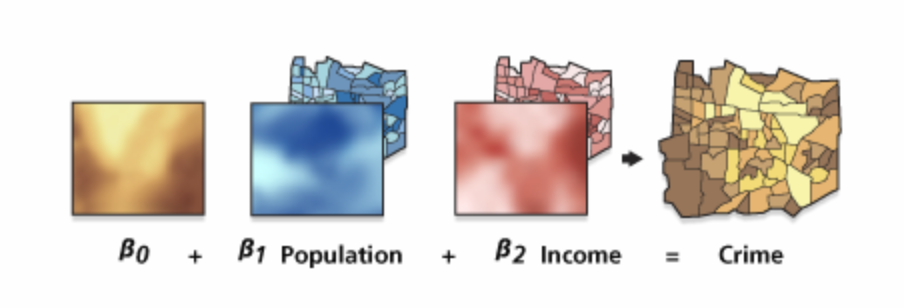
GWR is “a local form of linear regression used to model spatially varying relationships” (“Help”). Located under spatial statistics in ArcToolbox, I used this tool to perform a different form of linear regression on the crime vs. income & employment layer. It “constructs a separate equation for every feature in the dataset incorporating the dependent and explanatory variables of features falling within the bandwidth of each target feature” and is best used with data sets featuring several hundred features (“Help”). In my case, the data had several thousand which is okay because the more data the process has the better the output.