Hi everyone! As term 1 is nearing its end, I will be uploading parts of the labs I have been working on throughout the term. Throughout this course we have had a lot of hands on experience in lab, building our understanding of ArcGIS software, its uses and properties. I hope some of what I learned comes across in these posts, and I hope you enjoy the maps and final project that I have created along the way.
Coordinate Systems:
Coordinate Systems are basically arbitrary designations for spatial data. They provide a common basis for communication of a particular place or area on earth (for example, conic projections vs azimuthal projections). The reason why you can’t combine data with different coordinate systems to analyze it is that when data is projected into a different coordinate system, properties of Shape, Area, Distance and Direction can all be affected. In lab, we were given a number of misaligned or improperly referenced spatial data and we had to fix these in order to analyze the data properly. There are two methods to achieving this, both with distinct pros and cons:
- Projection on the fly: this is a built in feature of ArcMap, where the software makes it look like the two data layers are in the same coordinate system, when actually they may not be. Projecting on the fly also allows you to go into the properties of a layer and change the information in order to make this happen manually.
- Arc Toolbox: Project Command – While the above method works for display, for spatial analysis it is better to use Arc Toolbox’s ‘Project’ Command to actually go in an transform the data in order to create a new layer under a common spatial reference system.
Landsat Data:
What are the advantages of using remotely sensed data for geographic analysis?
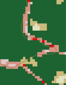
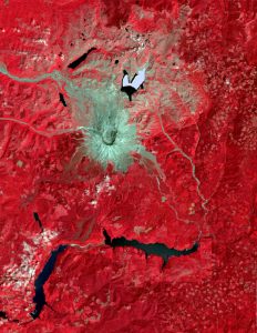
Landsat Data is basically data gathered using a satellite to scan and capture images of earths surface. This data can be very powerful, as, due to the nature of satellites in relation to earth, a very large number of images can be captured over a long time frame. This is great for large scale raster analysis; for example analyzing land use change over time. However, one disadvantage is the fact that because it is satellite imagery, localized analysis of features such as roads are inaccurate. This connects to the mixed pixel problem, which states that in raster at low resolution, all variation within a pixel is lost. I have included a number of images created in lab showing the pros and cons of this data. The image in red is a landsat analysis of landuse change for Mount St. Helens, while the green shows the mixed pixel problem at work; the vector line is the actual position of a road, while the pink and red raster pixels also represent the road; albeit a less accurate version from raster landsat data.