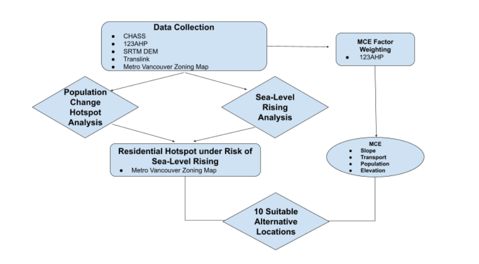
Figure 1: Flow chart of the project

Given that Metro Vancouver is a coastal municipality with several places with low sea levels, such as Richmond, which was built on islands in the delta of the Fraser River. In order to understand how the sea-level rise affects society and human well-being, it is effective and essential to use the GIS tool to analyze the impact of sea-level rise and advice for future investment and city development. 

The first step is data preparation. In order to produce a hotspot map of population change, CHASS data was obtained through UBC CWL for Metro Vancouver 2011 and 2016 populations. 

For sea-level-rise analysis, We obtained the DEM for the world from SRTM DEM then clipped it into the Metro Vancouver region. Metro Vancouver Zoning map is also used in our project to identify the hotspot areas. Since the residential areas have the most direct impact on human well-being and the focus of city development, such as facilities and infrastructures that are built around them, non-residential identified hotspot areas are not included in this project. 

For the purpose of searching alternative areas for the residential hotspot that is at risk of sea-level rise, four factors are defined for multiple criteria evaluation: population, slope, transport, and elevation. 123 AHP website was used to weigh each factor.

Hotspot Map Procedure

The second step is producing a hotspot map for Metro Vancouver’s population change between 2011 and 2016. After obtaining population data from the CHASS, the data was formulated and exported into the geodatabase, then joined with the Metro Vancouver shapefile. A field of population change between 2011 and 2016 was created, and the change was calculated by using ‘calculate field’ to subtract values of 2011 from 2016. Then optimized hotspot analysis was conducted to produce the map.

Figure 2: Screenshot of Example of population change column

Sea-Level-Rise Map Procedure

The third step is to evaluate the impact of sea-level rise. After Clipping the DEM to the Metro Vancouver area, ‘fill’ tool was applied to remove the imperfections in the
original DEM to overcome the sink problem, which converted the negative cell values into
meaningful elevations. Next, a ‘raster calculator was used to extract desired cells of 1 meter and 5 meters to form a new raster. Because the obtained new rasters contain two values, with 1 representing the cells of interest and 0 representing the remaining, the ‘reclassify’ tool was then applied to reclassify the 0 value cells as No Data. Then the reclassified 1 meter and 5 meters sea-level-rise DEM were converted to vector data to form the sea-level-rise maps by using ‘raster to polygons.

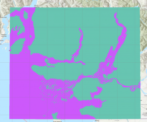
Figure 3: Screenshot of 5 m Sea-level rise raster before classification

Figure 4: Screenshot of Reclassified 5 m sea level rise raster

After obtaining a hotspot map and sea-level rise map, the next step is to determine the affected residential hotspot area. To achieve it, the ‘intersect’ tool was used for the generated two maps to locate the overlapped areas, representing the area under risk of 5-meter sea-level rise. When the intersection is produced, we compare the result with the Metro Vancouver zoning map to exclude the non-residential area, improving accuracy and reducing bias. The orange-red color hotspot at Coquitlam is a forest zone, and the one near the coast of Surrey is farmland. Only dark red-colored hotspot areas are considered residential zones, with a total of 1855345.7 m2.

Figure 5: Screenshot of intersection hotspot with a residential hotspot in dark red

After the total area of hotspots with the highest population change was calculated, the next step is to find the suitable areas for people who intend to move to consider as alternatives rather than move into the risk area. We consider conducting multiple criteria evaluation by using a suitability model to do so. There are 4 factors we consider an area is suitable for living: transport convenience, relatively low population density, the small slope for daily life and building construction, and safer/higher elevation. We think the elevation is much more critical than the slope; the elevation is more important than transport; the elevation is a bit more important than population density; the transport is more important than the slope; the population density is much more important than the slope; the transport is a bit more important than the population. The weighting of each factor is determined through the analytic hierarchy process through 123AHP website. The AHP result shows that the elevation, transport, population density, and slope weighed 50.88%, 25.69%, 18.53%, and 4.9%, respectively. Then a suitability model was applied, and each weight was input into the setting.

FIgure 6 & 7: AHP results

Suitability model procedures

For elevation data, since DEM was already raster form, it was imported into suitability model, using MSSall function with a lower threshold of 5 meters, representing that we want the alternative areas to be away from the risk area under extreme sea-level rise scenarios.

A heat map was first generated from Translink data using the ‘kernel density’ tool to convert data from vector to raster. Then the heat map was imported into a suitability model with inverse MSSall function, meaning areas closer to the public transport are favored.

For population data, the ‘feature to point’ tool was applied first on the 2016 population to create a new point feature class from the attribute table of Metro Vancouver, followed by the ‘kernel density’ tool to produce a raster heatmap. After that, the heatmap was imported into a suitability model to lower the population having a better suitability score.

For the slope data, the ‘slope operation’ spatial analyst tool was used on the Metro Vancouver DEM to generate the slope raster. Then the raster was imported into the suitability model, using MSSall function with an upper threshold of 20. It was suggested that anything above 0.2 is considered steep and will increase construction costs and difficulty (Legal Eagle Contractors Co, 2021).

After setting up the functions and weighting for each factor, a multiple criteria evaluation was conducted, and then a ‘locate’ tool in the suitability model was used to find 10 alternative areas with a total area of 1855345.7 m2. Besides, the best suitable location was located as well.

Figure 8: Screenshot of MCE results