Relevant factors for site suitability:
Through literature research we identified eight main factors that would impact site suitability for a new well. These were:
- Proximity to existing wells
- Underlying aquifer size and location
- Precipitation levels
- Water flow accumulation levels
- Slope
- Soil type
- Land use type, including distance from coastline
- Proximity to existing water pipelines
The justification for choosing these eight factors, and the methods we used in their analysis, are explained below.
Data sources:
- HectarsBC
- Precipitation
- Soil
- Slope – elevation (DEM)
- Sunshine Coast Regional District
- Water mains
- Coastline
- Government of British Columbia
- Wells
- Also, water depth data associated with wells used to determine aquifer size/location
- Wells
- Abacus Dataverse Network
- Land cover

![]()
![]()

Initial data conversions
To be able to work with all the different data together without issue, our first task was to convert the layers to the same coordinate system and datum as follows:
Geographic Coordinate System – NAD 1983 UTM Zone 10N
Datum – D North American 1983
In order to efficiently process the data we first had to limit the extent to our specific area of interest. This was done by drawing a circle around the town of Sechelt and then creating a 5 km buffer around that circle. We chose 5 km because this made sure to encompass a large enough area to allow us to meaningfully investigate the range of factors that would impact site suitability, but still small enough so that the data amount wouldn’t slow us down given the limitations to the computational power available to us. Additionally, having a larger area of interest would not necessarily add value to our investigation because we are looking to find a suitable site for a well to provide water to Sechelt, hence there is no need to look for sites too far from the town. The processing extent of the analysis was based upon this, and all layers that we imported were clipped to this area.
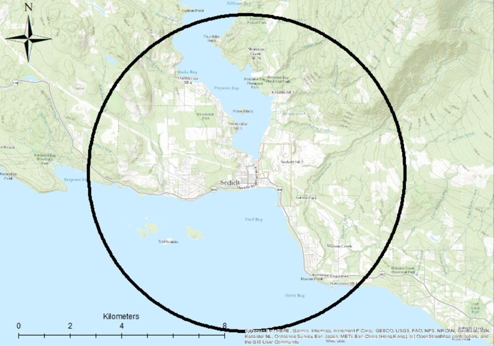
Spatial extent to our specific site of interest
Processing the layers
The following is a description of how each layer was processed and prepared for use in the multi-criteria analysis.
Wells:
The first layer that was processed was the existing wells. This layer contained information about the spatial distribution of the current wells in Sechelt as well as the depth of each well. According to the literature, a new well should not be placed within 15 meters of an existing well. This is to reduce interference between the wells, lessen the impact on the groundwater and limit the consequences of well contamination (Government of British Columbia, 2016). From the wells we therefore created a multiple-ring buffer of 15 m, 30 m, 45 m and 5000 m away from the buffer. The last ring was made very big to ensure we captured the rest of the area of interest. The buffer was then clipped within the 5 km circle around Sechelt as described above and converted into raster by ‘polygon to raster’ in order to reclassify it. The resolution selected was 5 m to ensure we retained adequate representation of the relatively small ring buffers, and the cell assignment method was selected to be ‘maximum cover’, which was done for all raster conversions in the project, because of the more direct link to the area coverage.
The buffer was then reclassified on a scale of 0 to 3, where 0 was assigned to areas that are unsuitable and therefore removed from the analysis, 1 assigned to areas with limited suitability and 3 to areas with most suitability.
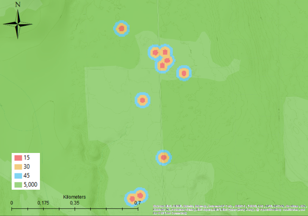
Buffers around existing wells
Aquifer:
We then went on to use information of water depth contained in the wells data to create a layer showing the underlying aquifer characteristics in order to determine the areas with higher water potential for the new well site.
The existing wells for which we had data were a wide range of depths and sizes and had a multitude of uses, from supplying only one or two people with water, to supplying a much larger population, as well as some wells not being used at all. The well we are interested in developing will be on a large scale, hence the applicability of the smaller wells in our analysis is limited and therefore were discounted. In order to deselect wells that aren’t being used and small private wells, the ‘search by attribute’ tool was used to identify all wells with a yield less than 5 gallons per minute and exported to create a new point layer.
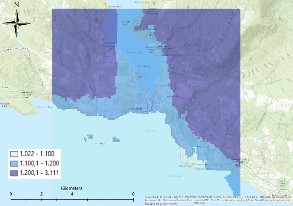
Next, we chose to use inverse distance weighted (IDW) interpolation to create the layer since this method estimates the cell value by averaging the data points, which is sufficient when considering the certainty of the data. We chose to carry out the interpolation to the power of 3 because of the relatively larger importance of the local area around each well, resulting from the highly variant spatial distribution of soils which are important in determining the underlying aquifer capacity. Additionally, the aquifers are affected by the permeability of the underlying bedrock which unfortunately we were unable to include in our analysis due to a lack of data. Following the creation of the aquifer layer, we reclassified the data from 1 to 3, where the greatest water depth is most suitable.
Underlying aquifer. Interpolated from well depth data
Precipitation:
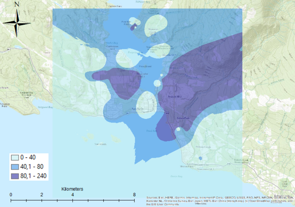
The precipitation layer was converted from vector to raster and collected into three groups: below 1100 mm (time period?), 1100-1200 mm and above 1200 mm. These groups were then reclassified respectively from 1 to 3, with the larger precipitation values suggesting a larger recharge of the underlying aquifer which would be beneficial for the well.
Precipitation levels
Water flow:
Leading from this, the amount of precipitation actually reaching the underlying aquifers is affected by surface conditions. A flow analysis was conducted to investigate this using the ‘Flow Direction’ tool. The option for multiple flow directions was assigned towards all down-slope neighbours from every cell of the DEM, meaning that the water could flow in multiple directions if multiple neighbouring cells had lower elevations, rather than just flowing straight down the cell with the overall lowest elevation; this was chosen as it avoids oversimplification and best represents the natural flow of water.
This flow direction layer was then used to create a ‘Flow Accumulation’ layer, which was a calculation of the number of cells that flow into a particular cell, thereby highlighting the areas where precipitation will accumulate. This layer was divided into 3 classes: 0 – 5 cells, 5 – 50 cells and above 50 cells. The class decisions were based on the large representation of cells with few cells running in to them, and therefore the classes are increasing towards the higher count. Finally the layer was reclassified in the same way as previous layers from 1 to 3, with 3 representing the largest precipitation accumulation.
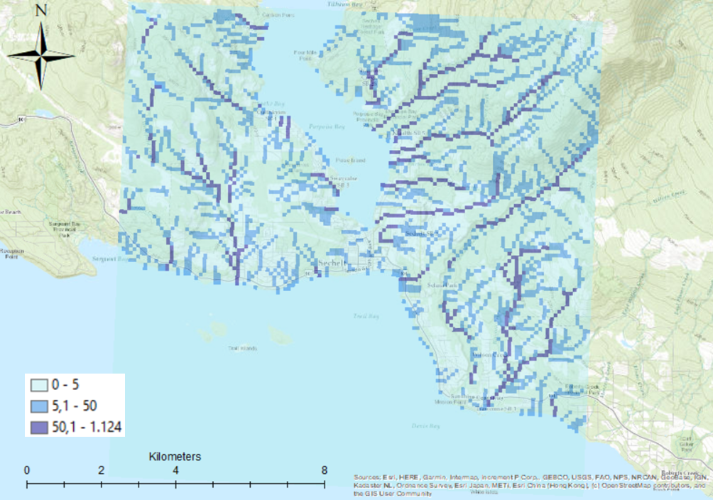
Areas of precipitation accumulation obtained from flow pathway analysis
Slope:
Following this, a slope layer was created from the DEM using the ‘Slope’ tool, based on the understanding that if a well is placed on a steep surface then the underlying water will flow away too quickly to be of use due to the gravity gradient. Three classes of gradients was created, 0-6 degrees, 6-12 degrees and above 12 degrees, which were then reclassified with the lowest gradient slopes being assigned 3. The justification for this classification was based on the spatial distribution of current wells compared to slopes, whereby existing wells tend to be situated on areas of low gradient.
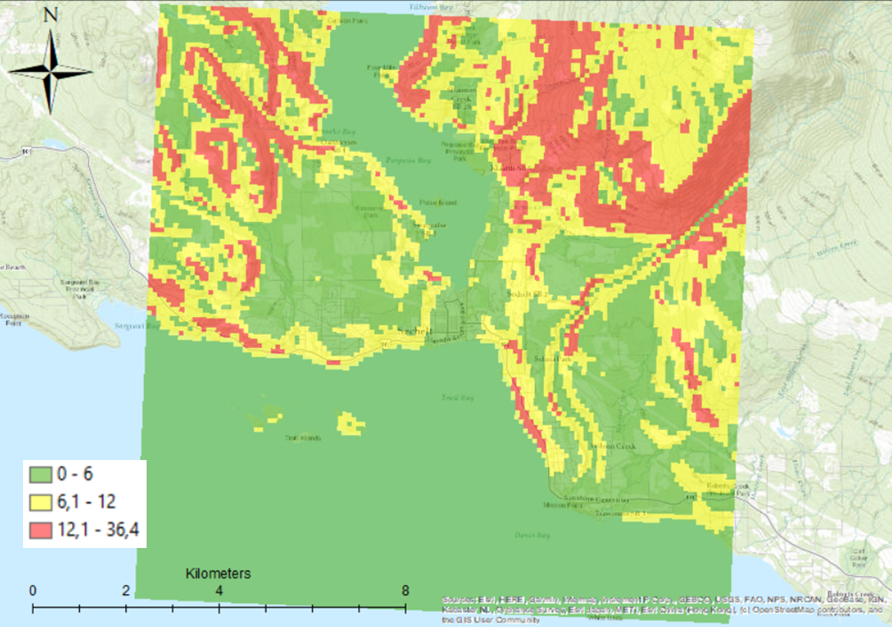
Slope gradients
Soil:
The soil layer was converted from vector to raster and classified into 3 groups 1-3, again with 3 representing the most suitable locations. This classification was based on both the spatial distribution of current wells and knowledge regarding the better materials for aquifers having higher porosity (Earle, 2015); most existing wells were found on either ‘loamy sand’ or ‘silty loam’ hence these two soil types were assigned 3 in the reclassification, sandy loam (which contained a few wells) was assigned 2 and loam (which contained the least wells) was assigned 1.
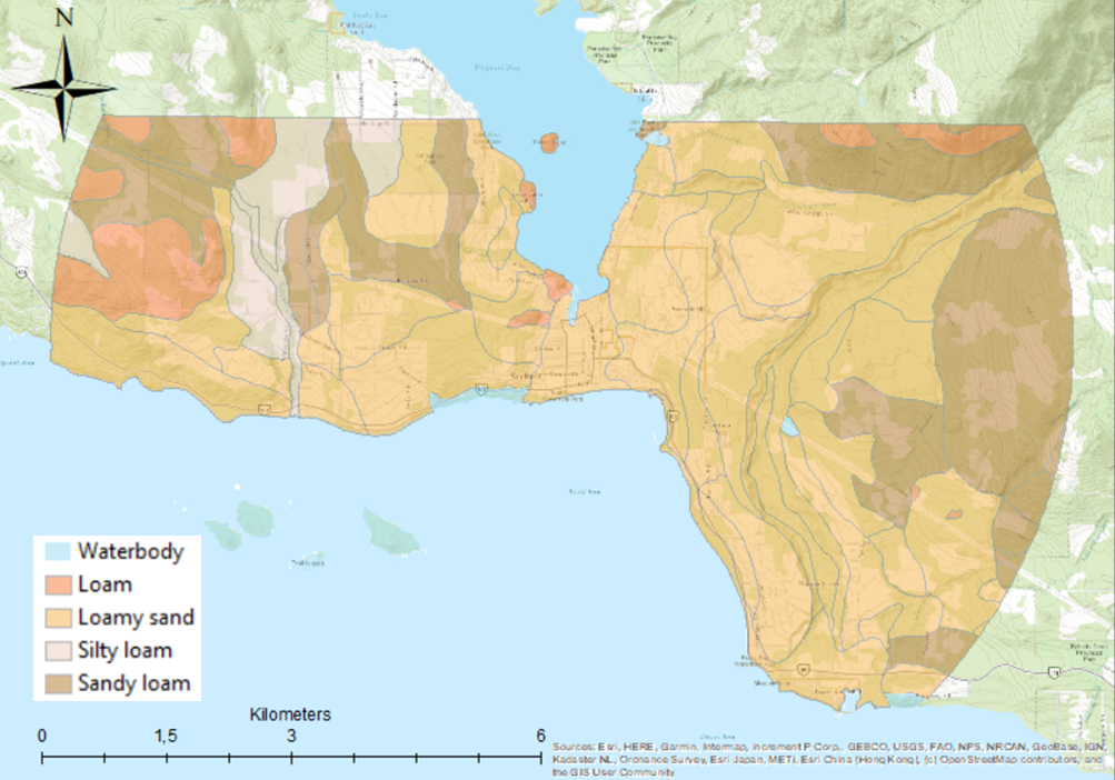
Spatial distribution of different soil types
Land cover:
The land cover map we were able to obtain only contained information regarding the urban areas in Sechelt, therefore an additional layer was created containing a buffer around the urban area to represent the open land. These two layers were then merged using the ‘Union’ tool.
After this, we created a coastline buffer to add to the land cover layer. This was done due to the growing issue of saltwater intrusion whereby pumping and well-drilling draws saline water into the freshwater aquifer, making the water undrinkable and leading to government recommendations to not drill new buffers within 50m of the coast (Government of British Columbia, 2016b). Accordingly, a buffer of 50 m was created, and this too merged with the new land cover map. When merging the two maps the coastal buffer map was ranked the highest due to the fact that the two maps would have different boundary areas and that we wanted to ensure the salt intrusion buffer was maintained. This layer, including different types of urban areas, open land and water bodies, was then converted to raster and reclassified where ‘open area’ was valued 3, ‘parks and recreational’ was valued 2, ‘residential’ was valued 1 and not excluded due to a few existing wells in these areas, and ‘waterbody’, ‘government and institutional’ and ‘resource and industrial’ were then valued 0 and excluded to avoid salt intrusion and because of the high cost and disadvantages (e.g. possible point pollution sources, or levels of disruption being too high) of placing a well here.
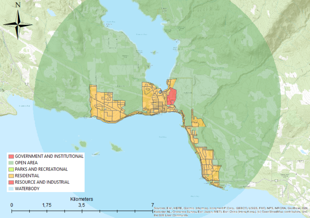
Different types of land cover
Existing water pipelines:
Finally, we wanted to consider proximity to existing water mains for the site of the new well as this would help to minimise construction costs and disruption. To do this, a multi-ring buffer was created with distances of 250 m, 500 m and 1000 m around the existing water mains, converted to a raster layer and then reclassified as above with 3 being the most suited.
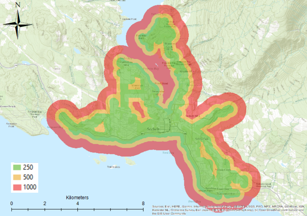
Multi-ring buffer around existing water pipelines
Multi Criteria Analysis
The first step in the process of constructing the MCE is to apply a weight to each of the factors so that it is possible to conduct a “Weighted Sum” analysis, which is a measure of how much importance should be given to each factor. The weights used are summarised in the table below.
| 20 % | Land cover |
| 20 % | Soil |
| 15 % | Wells |
| 15 % | Pipes |
| 10 % | IDW aquifer |
| 10 % | Slope |
| 5 % | Flow |
| 5 % | Precipitation |
Land cover and soil are the most important factors due to soil type directly impacting the capacity of the underlying aquifers, and land cover limiting the logistical possibility of establishing a new well in certain areas.
The layers for existing wells and pipelines were then valued as second-most important due to the fact that increasingly the distance from existing pipes will result in an increase in the price of establishment and connection of the new well to the water mains, and the actual distance from existing wells is also important in order to reduce stress on aquifers and the potential consequences of well contamination.
Following this, the aquifer layer was weighted 10%. Whilst this criteria is very important for the potential capacity of the new well, the fact that the data was obtained from an interpolation based on a broad range of data points makes it somewhat unreliable hence the weighting has been reduced accordingly. Slope was also weighted 10% due to the fact that the slopes classification is somewhat arbitrarily constructed and that it mostly affecting surface runoff.
Flow and precipitation were assigned the lowest weighting due to the fact that they are mostly impacting surface runoff, rather than aquifer recharge which is what we are more interested in for the well.
The weight scale was determined from the average of 12.5%, and then weighted above or below this average so that the sum of all factors equals 100%. The tool used to conduct the multi criteria evaluation was ‘weighted sum’ which multiplies the values of each classification so that areas with a value of 0 are removed from the analysis.
The results of the MCE were classified through standard deviation, with the top 10% displayed as the most suitable areas. The map is available in the ‘Results and Discussion’ page (available here).