Leaflet -R- Map | E-Portfolio of Stella L. Zhou

Data Processing:

This is a Leaflet -R-Map created for Vancouver’s Crime data in 2003 using R-studios programming.

*note: detailed data processing description will be towards the end of this page

Lost records of data

At the beginning I started of with 56952 data points for Vancouver crime data in 2003. After the process of parsing, geocoding and filtering, I ended up with 53425. The lost data are all from the two categories of “Homicide” and “Offence against person” because they do not have an address associated to them; hence during the process of geocoding, no coordinates can be assigned to their address column which was “Off Set to Protect Privacy”. Surprisingly I did not loose any data after I apply the boundary filter, this may indicate that all the data are already located within the city boundary, or possibly something wrong in my coding that didn’t filter out any outliers.

Data Error

In my opinion, there is quite a bit of error in this data since I had to take out 3527/56952 data points, which also happens to be two whole categories. This means that the final map isn’t representing the full Vancouver Crime Data in 2003 but only the ones that has a address associated to them. I could have kept those data and proceeded to geocoding, but all those 3527 data points will have the exact same co-ordinates; even if I offset them, their location will be randomly located and will not correctly represent the geospatial information as they should. Therefore I feel like keeping them would have a negative impact on the data integrity, because those 3527 data points will be misleading and confusing the audience on how those crime are distributed around the city.

Apart from this error, since most data points are present in hundreds block with “x” or “xx” substituted into the full address to protect privacy, they are also not representing their exact geospatial location. However, they are in proximity to the original location, so even after substituting “x” with “0”, the data representation is still close enough to the true data. In general, this data is more reliable for certain categories of crime than others due to the way their full addresses are recorded.

File Format

I am still a little confused by the different file format, but as far I know and learned in class, Shapefile was developed by ERSI for purpose to use in GIS software such as ArcGIS; whereas GeoJSON is a JavaScript object notation used to represent geospatial data information in formatted numbers, so it can be used in programming languages such as Rstudio. GeoJSON also doesn’t contain any styling information like the shapefile.

I converted my data into both shapefile and GeoJSON because I followed the tutorial and thought the shapefile might also come into use despite the fact I did not intend to use ArcGIS. This was true since I did have to use the shapefile when aggregating data to the hexagons using poly counts function. In the future, I might only need to convert data to shapefile or GeoJSON file only depending on what application I’m using and for what purpose. If I need to input this data to ArcGIS, I would definitely need to convert to shapfile since ArcGIS would not be able to read GeoJSON.

Visualisation Process:

Cartographic Design

It is pretty satisfying and visually pleasing to see an interactive map that you created with codes, however I do realize I’ve encountered many cartographic design due my limited coding skills. Unlike ArcGIS and Adobe Illustrator, I can not always see the visual changes I’ve made unless I print the map out every time I run a code. This makes it harder when you want to see all the changes you’ve made over time and adjust accordingly. In addition, I didn’t know how to pick more specific colours other than using the basic colour names. I am so used to using software such as ArcGIS and Adobe creative suite where I can visualise everything on my work space, hence trying to incorporate more complicated visual designs on Rstudio was very difficult. I am wish I was able to add more visual features or adjust the colour choice more, but I did not know how to do so within the time I had. In this case, I would have preferred using ArcGIS or Adobe Illustrator to represent and refine my map.

Some things I did change in my code is the colour choice and radius of circle markers. I try to associate the type of crime with the type of land use. For example I used yellow for residences and red for commercial break in because they are usually the colours the use on zoning maps. At first I also changed the radius to 4 instead of using 2 since they are easier to click on when zoomed in; however I changed it back to 2 because I realized that I did not combine any categories together, so it isn’t necessary for the audience to click on each data points in order to tell which crime it represents. Using radius 2 gives a good distribution map of the crime without overcrowding the base map areas.

Reflection on using R-studio:

After using both expensive proprietary software packages such as ArcGIS and Adobe Illustrator, and free opensource programming language such as processing and Rstudio, I have a better understanding of both ends.

For ArcGIS and Adobe Illustrator, they are very good tools for the actual data representing part of the data visualisation pipeline. You can visually see all the changes you make during the whole process, and you can easily pick and customise your visual elements. You may also do data mining and parsing on ArcGIS using the “select by attribution” function. These functions make ArcGIS and Adobe creative suite visually intuitive to use. However, data mining and filtering process can be long and complicated on Arc when you have massive data set. In addition, the high cost to access ArcGIS and Adobe creative suite makes them less public friendly.

On the other hand, free opensource programming tools such as Rstudio and leaflet is pretty commonly use by the public. They are faster in executing the data mining & filtering processes especially if you have massive geospatial data sets such as Vancouver Crime data. Since geospatial data information is stored as numbers, it also takes up far less storage space on your device. However, if you are limited in your coding skills, it can be very hard to trouble shoot issues as they occur. Although there are lots of communities online in which you can get help from, but it is also hard to judge whether a solution pertains to your situation in particular.

Emotionally, I can be bias towards proprietary software because they are the first ones I learned how to use even before taking a course in GIS (especially adobe). Therefore although I get frustrated when I encounter problems both in proprietary mapping soft ware and open source programming languages, I find myself more irritated in the latter situation. For ArcGIS and Adobe, they are easier for me to trouble shoot because I have previous knowledge and can play around with them easily; however due to my very limited skills and experience with programming, I suffered a lot when encountering small issues and have to go to my TA in person more than once to get unstuck on certain steps.

Step by step Data Processing:

First step: downloading the data and extract

The first thing I did with the downloaded data was to extract only the year I want, which is 2003. This resulted in 56,952 data points.

I also noticed that two categories do not have any address assigned, instead they have “Off Set to Protect Privacy”. I decided take the two categories (“homicide” & “offence against person”) out of the data set in order to decrease geocoding time, since it would not be possible to correctly geocode these data in the first place. Most likely they will end up showing as one location on the map; even if I offset every single point data for those two category, I will be assigning them incorrect locations that are still clustered together. Although both ways decreases the integrity of this data set, I still choose to take those two categories out instead of leaving it in. It is better to not present these data instead of having them clustered at one location on the map, making it confusing or misleading for the audience.

In the end, the total number of data points I read into R to geocode is 53,425.

Acquire Data in Rstudio

After loading the library I acquired the data from my extracted csv file and printed out the head data to inspect.

######################################################
# Vancouver VPD: Crime Data Processing Script
# Date: October 2016
# By: Stella Z.
# Desc: Data filtering for VPD Crime Data 2003
######################################################

# Instal neede libraries
install.packages("GISTools")
install.packages("RJSONIO")
install.packages("rgdal")
install.packages("RCurl")
install.packages("curl")

#Load libraries
library(GISTools)
library(RJSONIO)
library(rgdal)
library(RCurl)
library(curl)

#-------------------------------------------------------------#
#----------------Acquire Data from CSV------------------------#
#-------------------------------------------------------------#

#set file name and location
fname ='C:\\Users\\Stella~\\Desktop\\Rmap\\VPDcrimedata2003geocode.csv'

# Read data as csv into R
data = read.csv(fname, header=T)

# inspect data
print(head(data))

Parse Data

Then I substitute all the “X” in the address for “0”, and created a new column to show the hundred block address full numbers. I also added a new full address column that connected the new h_block with “Vancouver, BC” at the end.

#-------------------------------------------------------------#
#----------------Parse data in csv 2003-----------------------#
#-------------------------------------------------------------#

# change intersection from ## to 00's
# create new h_block column
data$h_block = gsub("X", "0", data$HUNDRED_BLOCK)
print(head(data$h_block))

# Creat new 'full_address' column & add "Vancouver, BC":
data$full_address = paste(data$h_block,
                          "Vancouver, BC",
                          sep=", ")

# write file out
ofile = "C:\\Users\\Stella~\\Desktop\\Rmap\\VPDcrimedata2003workfile.csv" 
write.csv(data, ofile)

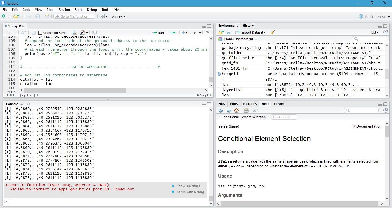
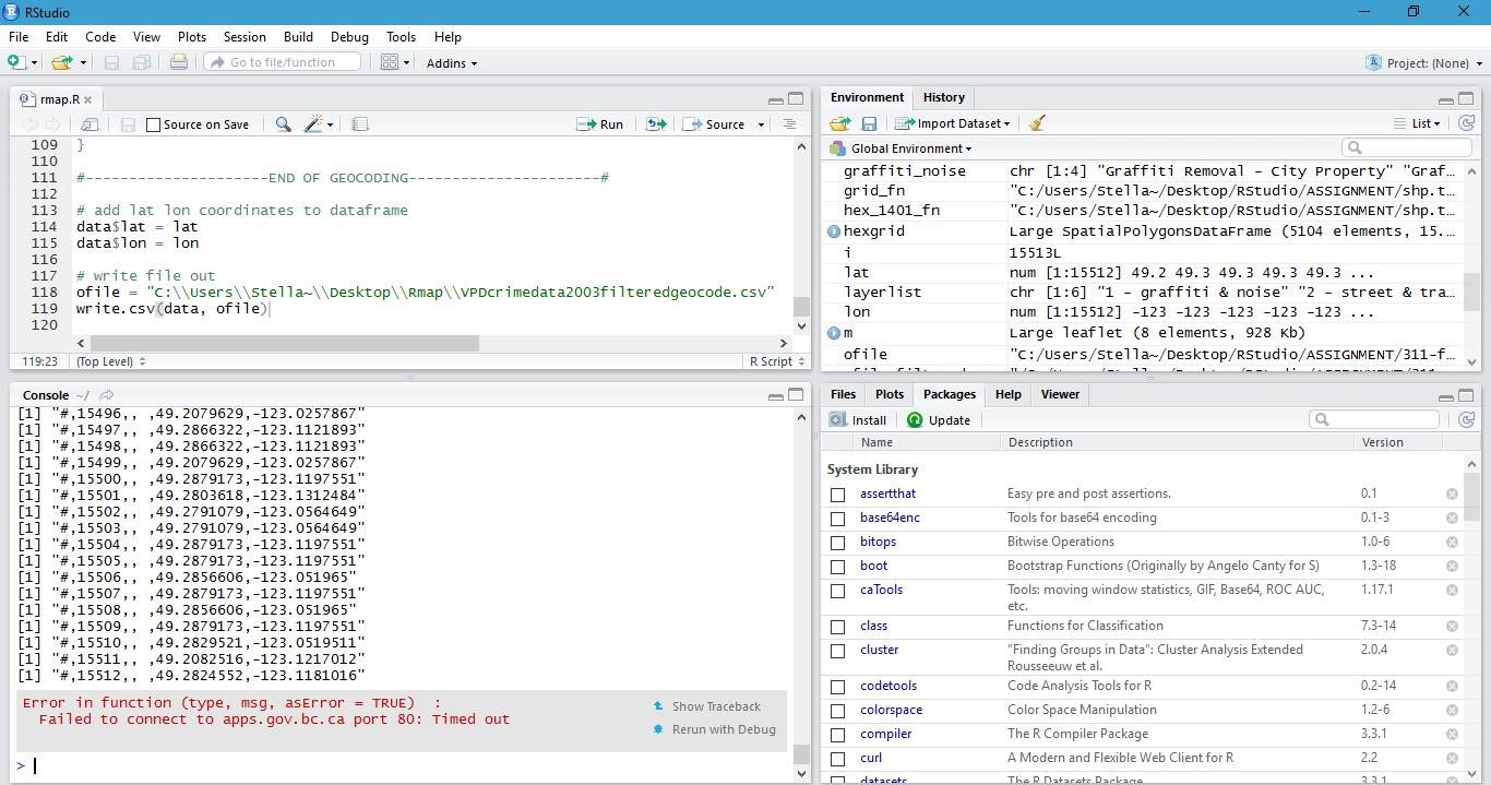
Although the next step is to geocode all the data, I was never successful in completing this step. My code was correct and it ran smoothly, yet my full dataset was not able to successfully geocode. Every time it would fail sometime during the process and stop geocoding the remaining data, and I would have to start over. This is probably due to R loosing connection with the BC government geocoding API website. After 6 trials and over 30hrs of trying, Rstudio still cannot fully geocode the massive amount of data I have. At first I thought it might have been my internet problem at home, but I also tried it at a coffee shop and on UBC campus, they still failed. To this point I am still not clear whether it is my laptop’s issue or simply unstable internet connection to the BC government server; but it is something to put in mind in the future when I have to geocode such massive datasets. In the end I had to seek help from Andras, and I was able to obtain the geocoded data from him in order to proceed to my next step. Here I will post screen shots of 2 out of 6 trials that did not work out:

Data Mining

The next part is Data mining. I searched for all the case group in this data set, which is the different categories of crime. 6 classes were returned. Because they are only 6 classes and the titles are relatively clear and descriptive, I decided to keep them and not generalise them into fewer classes.

#-------------------------------------------------------------#
#------------------------Data Mining--------------------------#
#-------------------------------------------------------------#

# examine the types of cases - Print each unique case on a new line for easier inspection
for (i in 1:length(unique(data$TYPE))){
  print(unique(data$TYPE)[i], max.levels=0)
}

#Result in the following groups
#[1] Break and Enter Residential or Other
#[1] Theft of Vehicle
#[1] Other Theft
#[1] Theft from Vehicle
#[1] Break and Enter Commercial
#[1] Mischief
#Only 6 classes and they are all quite clear
#decide to keep all 6 classes in its original titles

Then I put each class into vectors in order to assign CID to each of them.

#-----------------Putting class into vectors-------------#

# Break and Enter Residential or Other
Break_and_Enter_Residential_or_Other = c('Break and Enter Residential or Other')

# Theft of Vehicle
Theft_of_Vehicle = c('Theft of Vehicle')

# Other Theft
Other_Theft = c('Other Theft')

# Theft from Vehicle
Theft_from_Vehicle = c('Theft from Vehicle')

# Break and Enter Commercial
Break_and_Enter_Commercial = c('Break and Enter Commercial')

# Mischief
Mischief = c('Mischief')

#-------------------Assignning CID-----------------------#

# give class id numbers:
data$cid = 9999
for(i in 1:length(data$TYPE)){
  if(data$TYPE[i] %in% Break_and_Enter_Residential_or_Other){
    data$cid[i] = 1    
  }else if(data$TYPE[i] %in% Theft_of_Vehicle){
    data$cid[i] = 2   
  }else if(data$TYPE[i] %in% Other_Theft){
    data$cid[i] = 3   
  }else if(data$TYPE[i] %in% Theft_from_Vehicle){
    data$cid[i] = 4   
  }else if(data$TYPE[i] %in% Break_and_Enter_Commercial){
    data$cid[i] = 5   
  }else if(data$TYPE[i] %in% Mischief){
    data$cid[i] = 6  
  }else{
    data$cid[i] = 0   
  }
}

Then I offset data points that might overlap. Since I substituted “X” with “0”, there is the possibility that some hundred block addresses are geocoded to the exact same location. Therefore running this loop will offset the same data points slightly away from the original point.

#-------------handingling overlaping points if any---------------#

# Set offset for points in same location:
data$lat_offset = data$lat
data$lon_offset = data$lon

# Run loop - if value overlaps, offset it by a random number
for(i in 1:length(data$lat)){
  if ( (data$lat_offset[i] %in% data$lat_offset) && (data$lon_offset[i] %in% data$lon_offset)){
    data$lat_offset[i] = data$lat_offset[i] + runif(1, 0.0001, 0.0005)
    data$lon_offset[i] = data$lon_offset[i] + runif(1, 0.0001, 0.0005)
  } 
}

Last step of my data mine was to filter out data that might lie outside the City of Vancouver boundary. However, after this step my data points remained the same. Which could either mean there isn’t any outliers, or there could have been an error somewhere in the code. I wrote out the newly filtered CSV out so I don’t loose all the data.

# ---------------------------- Filter ------------------------------ #

# Filter outdata that are outside vancouver boundary
data_filter = subset(data, (lat <= 49.313162) & (lat >= 49.199554) & 
                       (lon <= -123.019028) & (lon >= -123.271371) & is.na(lon) == FALSE )
# plot the data
plot(data_filter$lon, data_filter$lat)

# write file out for filtered data
ofile = "C:\\Users\\Stella~\\Desktop\\Rmap\\VPDcrimedata2003workfile_filtered.csv" 
write.csv(data, ofile)

Converting Data into Shape files and Geojson files

I saved the data into Shape files and Geojson files so I can use later in making the leaflet map. I also named them according to the data set so I am able to find them easily later to use.

# ------------------------------------------------------------------ #
# ---------------------Saving Data Sets ---------------------------- #
# ------------------------------------------------------------------ #

# -------------------- Convert Data to Shapefile-------------------- #

# store coordinates in dataframe
coords_crime = data.frame(data_filter$lon_offset, data_filter$lat_offset)

# create spatialPointsDataFrame
data_shp = SpatialPointsDataFrame(coords = coords_crime, data = data_filter)

# set the projection to wgs84
projection_wgs84 = CRS("+proj=longlat +datum=WGS84")
proj4string(data_shp) = projection_wgs84

# set an output folder for our geojson files:
geofolder = "C:\\Users\\Stella~\\Desktop\\Rmap\\final\\"

# Join the folderpath to each file name:
opoints_shp = paste(geofolder, "crime_", "2003", ".shp", sep = "")
print(opoints_shp) 

opoints_geojson = paste(geofolder, "crime_", "2003", ".geojson", sep = "") 
print(opoints_geojson)

# write the file to a shp
writeOGR(data_shp, opoints_shp, layer = "data_shp", driver = "ESRI Shapefile",
         check_exists = FALSE)

# write file to geojson
writeOGR(data_shp, opoints_geojson, layer = "data_shp", driver = "GeoJSON",
         check_exists = FALSE)

Before moving onto leaflet, I aggregate the data to hexagon grids. I took the blank hexagon frame file from Andras (since Joey’s website wasn’t working) and transformed the projection to wgs84. Next I assigned value to it by using the poly.count function, which calculates the number of crime per grid cell. Then I also write this out as shape and geojson files for later use.

# ------------------------------------------------------------------ #
# ---------------------Creating Hexagon Grid ----------------------- #
# ------------------------------------------------------------------ #

# ------------------- aggregate to a grid -------------------------- #
# ref: http://www.inside-r.org/packages/cran/GISTools/docs/poly.counts
grid_fn = 'C:\\Users\\Stella~\\Desktop\\Rmap\\blank_hex.geojson'

# read in the hex grid setting the projection to utm10n
hexgrid = readOGR(grid_fn, 'OGRGeoJSON')

# transform projection to wgs84 to match point file and store it to a new variable
hexgrid_wgs84 = spTransform(hexgrid, projection_wgs84)

#------------------Assigning Value to Hex Grid-----------------------#
# count the number of occurrences of crime per grid cell
grid_cnt = poly.counts(data_shp, hexgrid_wgs84)

# define the output names:
ohex_shp = paste(geofolder, "hexgrid_", "crimedata2003", "_cnts",".shp", sep = "")
print(ohex_shp)

ohex_geojson = paste(geofolder, "hexgrid_", "crimedata2003", "_cnts",".geojson", sep = "") 
print(ohex_geojson)

# write the file to a shp
writeOGR(check_exists = FALSE, hexgrid_wgs84, ohex_shp, 
         layer = "hexgrid_wgs84", driver = "ESRI Shapefile")

# write file to geojson
writeOGR(check_exists = FALSE, hexgrid_wgs84, ohex_geojson, 
         layer = "hexgrid_wgs84", driver = "GeoJSON")

##############END OF DATA PROCESSING##################

This is the end of stage of data processing for Vancouver Crime data 2003

My Full Code Script in Rstudio:

######################################################
# Vancouver VPD: Crime Data Processing Script
# Date: October 2016
# By: Stella Z.
# Desc: Data filtering for VPD Crime Data 2003
######################################################

# Instal neede libraries
install.packages("GISTools")
install.packages("RJSONIO")
install.packages("rgdal")
install.packages("RCurl")
install.packages("curl")

#Load libraries
library(GISTools)
library(RJSONIO)
library(rgdal)
library(RCurl)
library(curl)

#-------------------------------------------------------------#
#----------------Acquire Data from CSV------------------------#
#-------------------------------------------------------------#

#set file name and location
fname ='C:\\Users\\Stella~\\Desktop\\Rmap\\VPDcrimedata2003geocode.csv'

# Read data as csv into R
data = read.csv(fname, header=T)

# inspect data
print(head(data))

#-------------------------------------------------------------#
#----------------Parse data in csv 2003-----------------------#
#-------------------------------------------------------------#

# change intersection from ## to 00's
# create new h_block column
data$h_block = gsub("X", "0", data$HUNDRED_BLOCK)
print(head(data$h_block))

# Creat new 'full_address' column & add "Vancouver, BC":
data$full_address = paste(data$h_block,
                          "Vancouver, BC",
                          sep=", ")

# write file out
ofile = "C:\\Users\\Stella~\\Desktop\\Rmap\\VPDcrimedata2003workfile.csv" 
write.csv(data, ofile)

#-------------------------------------------------------------#
#------------------------Please Note--------------------------#
#-------------------------------------------------------------#
#Geocoding process is omitted becasuse my laptop 
#failed to complete the process over 6 tirals
#the csv is a geocoded file from Andras
#-------------------------------------------------------------#
#-------------------------------------------------------------#

#-------------------------------------------------------------#
#------------------------Data Mining--------------------------#
#-------------------------------------------------------------#

# examine the types of cases - Print each unique case on a new line for easier inspection
for (i in 1:length(unique(data$TYPE))){
  print(unique(data$TYPE)[i], max.levels=0)
}

#Result in the following groups
#[1] Break and Enter Residential or Other
#[1] Theft of Vehicle
#[1] Other Theft
#[1] Theft from Vehicle
#[1] Break and Enter Commercial
#[1] Mischief
#Only 6 classes and they are all quite clear
#decide to keep all 6 classes in its original titels

#-----------------Putting class into vectors-------------#

# Break and Enter Residential or Other
Break_and_Enter_Residential_or_Other = c('Break and Enter Residential or Other')

# Theft of Vehicle
Theft_of_Vehicle = c('Theft of Vehicle')

# Other Theft
Other_Theft = c('Other Theft')

# Theft from Vehicle
Theft_from_Vehicle = c('Theft from Vehicle')

# Break and Enter Commercial
Break_and_Enter_Commercial = c('Break and Enter Commercial')

# Mischief
Mischief = c('Mischief')

#-------------------Assignning CID-----------------------#

# give class id numbers:
data$cid = 9999
for(i in 1:length(data$TYPE)){
  if(data$TYPE[i] %in% Break_and_Enter_Residential_or_Other){
    data$cid[i] = 1    
  }else if(data$TYPE[i] %in% Theft_of_Vehicle){
    data$cid[i] = 2   
  }else if(data$TYPE[i] %in% Other_Theft){
    data$cid[i] = 3   
  }else if(data$TYPE[i] %in% Theft_from_Vehicle){
    data$cid[i] = 4   
  }else if(data$TYPE[i] %in% Break_and_Enter_Commercial){
    data$cid[i] = 5   
  }else if(data$TYPE[i] %in% Mischief){
    data$cid[i] = 6  
  }else{
    data$cid[i] = 0   
  }
}

#-------------handingling overlaping points if any---------------#

# Set offset for points in same location:
data$lat_offset = data$lat
data$lon_offset = data$lon

# Run loop - if value overlaps, offset it by a random number
for(i in 1:length(data$lat)){
  if ( (data$lat_offset[i] %in% data$lat_offset) && (data$lon_offset[i] %in% data$lon_offset)){
    data$lat_offset[i] = data$lat_offset[i] + runif(1, 0.0001, 0.0005)
    data$lon_offset[i] = data$lon_offset[i] + runif(1, 0.0001, 0.0005)
  } 
}

# ---------------------------- Filter ------------------------------ #

# Filter outdata that are outside vancouver boundary
data_filter = subset(data, (lat <= 49.313162) & (lat >= 49.199554) & 
                       (lon <= -123.019028) & (lon >= -123.271371) & is.na(lon) == FALSE )
# plot the data
plot(data_filter$lon, data_filter$lat)

# write file out for filtered data
ofile = "C:\\Users\\Stella~\\Desktop\\Rmap\\VPDcrimedata2003workfile_filtered.csv" 
write.csv(data, ofile)

# ------------------------------------------------------------------ #
# ---------------------Saving Data Sets ---------------------------- #
# ------------------------------------------------------------------ #

# -------------------- Convert Data to Shapefile-------------------- #

# store coordinates in dataframe
coords_crime = data.frame(data_filter$lon_offset, data_filter$lat_offset)

# create spatialPointsDataFrame
data_shp = SpatialPointsDataFrame(coords = coords_crime, data = data_filter)

# set the projection to wgs84
projection_wgs84 = CRS("+proj=longlat +datum=WGS84")
proj4string(data_shp) = projection_wgs84

# set an output folder for our geojson files:
geofolder = "C:\\Users\\Stella~\\Desktop\\Rmap\\final\\"

# Join the folderpath to each file name:
opoints_shp = paste(geofolder, "crime_", "2003", ".shp", sep = "")
print(opoints_shp) 

opoints_geojson = paste(geofolder, "crime_", "2003", ".geojson", sep = "") 
print(opoints_geojson)

# write the file to a shp
writeOGR(data_shp, opoints_shp, layer = "data_shp", driver = "ESRI Shapefile",
         check_exists = FALSE)

# write file to geojson
writeOGR(data_shp, opoints_geojson, layer = "data_shp", driver = "GeoJSON",
         check_exists = FALSE)

# ------------------------------------------------------------------ #
# ---------------------Creating Hexagon Grid ----------------------- #
# ------------------------------------------------------------------ #

# ------------------- aggregate to a grid -------------------------- #
# ref: http://www.inside-r.org/packages/cran/GISTools/docs/poly.counts
grid_fn = 'C:\\Users\\Stella~\\Desktop\\Rmap\\blank_hex.geojson'

# read in the hex grid setting the projection to utm10n
hexgrid = readOGR(grid_fn, 'OGRGeoJSON')

# transform projection to wgs84 to match point file and store it to a new variable
hexgrid_wgs84 = spTransform(hexgrid, projection_wgs84)

#------------------Assigning Value to Hex Grid-----------------------#
# count the number of occurrences of crim per grid cell
grid_cnt = poly.counts(data_shp, hexgrid_wgs84)

# define the output names:
ohex_shp = paste(geofolder, "hexgrid_", "crimedata2003", "_cnts",".shp", sep = "")
print(ohex_shp)

ohex_geojson = paste(geofolder, "hexgrid_", "crimedata2003", "_cnts",".geojson", sep = "") 
print(ohex_geojson)

# write the file to a shp
writeOGR(check_exists = FALSE, hexgrid_wgs84, ohex_shp, 
         layer = "hexgrid_wgs84", driver = "ESRI Shapefile")

# write file to geojson
writeOGR(check_exists = FALSE, hexgrid_wgs84, ohex_geojson, 
         layer = "hexgrid_wgs84", driver = "GeoJSON")

##############END OF DATA PROCESSING##################
######################################################
# Vancouver VPD: Leaflet map making
# Date: October 2016
# By: Stella Z.
# Desc: Composing Leaflet map for VPD Crime Data 2003
######################################################

# install the leaflet library
install.packages("leaflet")

# add the leaflet library to your script
library(leaflet)

# initiate the leaflet instance and store it to a variable
m = leaflet()

# add map tiles - default openstreetmap
m = addTiles(m)

#------------------Read processed data CSV file----------------------#

filename = "C:\\Users\\Stella~\\Desktop\\Rmap\\VPDcrimedata2003workfile_filtered.csv"
data_filter = read.csv(filename, header = TRUE)

# subset out data_filter:
df_Break_and_Enter_Residential_or_Other = subset(data_filter, cid == 1)
df_Theft_of_Vehicle = subset(data_filter, cid == 2)
df_Other_Theft = subset(data_filter, cid == 3)
df_Theft_from_Vehicle = subset(data_filter, cid == 4)
df_Break_and_Enter_Commercial = subset(data_filter, cid == 5)
df_Mischief = subset(data_filter, cid == 6)



# ----------------------------------------------------------------------- #
#------------------adding the colored circles to map----------------------#
# ----------------------------------------------------------------------- #

#add colour factors
colorFactors = colorFactor(c('orange', 'blue', 'red', 'green', 'purple', 'pink'),
                           domain = data_filter$cid)

#add circle markes for each layer
m = addCircleMarkers(m, 
                     lng = df_Break_and_Enter_Residential_or_Other$lon_offset, 
                     lat = df_Break_and_Enter_Residential_or_Other$lat_offset,
                     popup = df_Break_and_Enter_Residential_or_Other$TYPE, 
                     radius = 3, 
                     stroke = FALSE, 
                     fillOpacity = 0.75, 
                     color = colorFactors(df_graffiti_noise$cid),
                     group = "1 - Break and Enter Residential or Other")

m = addCircleMarkers(m, 
                     lng = df_Theft_of_Vehicle$lon_offset, 
                     lat = df_Theft_of_Vehicle$lat_offset, 
                     popup = df_Theft_of_Vehicle$TYPE, 
                     radius = 3, 
                     stroke = FALSE, fillOpacity = 0.75,
                     color = colorFactors(df_Theft_of_Vehicle$cid),
                     group = "2 - Theft of Vehicle")

m = addCircleMarkers(m, 
                     lng = df_Other_Theft$lon_offset, 
                     lat = df_Other_Theft$lat_offset, 
                     popup = df_Other_Theft$TYPE, 
                     radius = 3, 
                     stroke = FALSE, fillOpacity = 0.75,
                     color = colorFactors(df_Other_Theft$cid),
                     group = "3 - Other Theft")

m = addCircleMarkers(m, 
                     lng = df_Theft_from_Vehicle$lon_offset, 
                     lat = df_Theft_from_Vehicle$lat_offset, 
                     popup = df_Theft_from_Vehicle$TYPE, 
                     radius = 3, 
                     stroke = FALSE, fillOpacity = 0.75,
                     color = colorFactors(df_Theft_from_Vehicle$cid),
                     group = "4 - Theft from Vehicle")

m = addCircleMarkers(m, 
                     lng = df_Break_and_Enter_Commercial$lon_offset, 
                     lat = df_Break_and_Enter_Commercial$lat_offset, 
                     popup = df_Break_and_Enter_Commercial$TYPE, 
                     radius = 3, 
                     stroke = FALSE, fillOpacity = 0.75,
                     color = colorFactors(df_Break_and_Enter_Commercial$cid),
                     group = "5 - Break and Enter Commercial")

m = addCircleMarkers(m, 
                     lng = df_Mischief$lon_offset, 
                     lat = df_Mischief$lat_offset, 
                     popup = df_Mischief$TYPE, 
                     radius = 3, 
                     stroke = FALSE, fillOpacity = 0.75,
                     color = colorFactors(df_Mischief$cid),
                     group = "6 - Mischief")

#------------------add other basemap options----------------------#

m = addTiles(m, group = "OSM (default)") 
m = addProviderTiles(m,"Stamen.Toner", group = "Toner")
m = addProviderTiles(m, "Stamen.TonerLite", group = "Toner Lite")


#add layer controls to map
m = addLayersControl(m,
                     baseGroups = c("Toner Lite","Toner"),
                     overlayGroups = c("1 - Break and Enter Residential or Other", "2 - Theft of Vehicle",
                                       "3 - Other Theft","4 - Theft from Vehicle", "5 - Break and Enter Commercial",
                                       "6 - Mischief")
)

#make map to see map
m

# ----------------------------------------------------------------------- #
#--------------------------create Toggle Map------------------------------#
# ----------------------------------------------------------------------- #

# Put variables into list to loop:
data_filterlist = list(df_Break_and_Enter_Residential_or_Other = subset(data_filter, cid == 1),
                       df_Theft_of_Vehicle = subset(data_filter, cid == 2),
                       df_Other_Theft = subset(data_filter, cid == 3),
                       df_Theft_from_Vehicle = subset(data_filter, cid == 4),
                       df_Break_and_Enter_Commercial = subset(data_filter, cid == 5),
                       df_Mischief = subset(data_filter, cid == 6))

layerlist = c("1 - Break and Enter Residential or Other", "2 - Theft of Vehicle",
              "3 - Other Theft","4 - Theft from Vehicle", "5 - Break and Enter Commercial",
              "6 - Mischief")

# same color variable:
colorFactors = colorFactor(c('orange', 'blue', 'red', 'green', 'purple', 'pink'),domain = data_filter$cid)

# Creat loop to add markers to map object:
for (i in 1:length(data_filterlist)){
  m = addCircleMarkers(m, 
                       lng=data_filterlist[[i]]$lon_offset,
                       lat=data_filterlist[[i]]$lat_offset, 
                       popup=data_filterlist[[i]]$Case_Type, 
                       radius=3,
                       stroke = FALSE, 
                       fillOpacity = 0.75,
                       color = colorFactors(data_filterlist[[i]]$cid),
                       group = layerlist[i]
  )
}

#flip “overlayGroups” and “baseGroups”:
m = addTiles(m, "Stamen.TonerLite", group = "Toner Lite") 
m = addLayersControl(m,
                     overlayGroups = c("Toner Lite"),
                     baseGroups = layerlist
)

#view map
m

# ----------------------------------------------------------------------- #
#--------------------putting data into hexagon frame----------------------#
# ----------------------------------------------------------------------- #

library(rgdal)
library(GISTools)

# define the filepath
hex_crime_fn = 'C:\\Users\\Stella~\\Desktop\\Rmap\\final\\hexgrid_crimedata2003_cnts.geojson'

# read in the geojson
hex_crime = readOGR(hex_crime_fn, "OGRGeoJSON")

#initiate new map object with new toner
m = leaflet()
m = addProviderTiles(m, "Stamen.TonerLite", group = "Toner Lite")

# Create a continuous palette function
pal = colorNumeric(
  palette = "Greens",
  domain = hex_crime$data
)

# add the polygons to the map
m = addPolygons(m, 
                data = hex_crime,
                stroke = FALSE, 
                smoothFactor = 0.2, 
                fillOpacity = 1,
                color = ~pal(hex_crime$data),
                popup = paste("Number of crimes: ", hex_crime$data, sep="")
)

#add legend to map
m = addLegend(m, "bottomright", pal = pal, values = hex_crime$data,
              title = "VPD crime density",
              labFormat = labelFormat(prefix = " "),
              opacity = 0.75
)

m

#-------------------------------------------------------------#
#------------------------Please Note--------------------------#
#-------------------------------------------------------------#
#failed to produce hex polygon density map
#hence did not proceed to put point layer and hex grid together
#-------------------------------------------------------------#
#------------------------Please Note--------------------------#
#-------------------------------------------------------------#

###########################END OF MAPMAKNG###########################